Artificial intelligence (AI), sometimes called machine intelligence, is intelligence demonstrated by machines, unlike the natural intelligence displayed by humans and animals. Leading AI textbooks define the field as the study of “intelligent agents“: any device that perceives its environment and takes actions that maximize its chance of successfully achieving its goals. Colloquially, the term “artificial intelligence” is often used to describe machines (or computers) that mimic “cognitive” functions that humans associate with the human mind, such as “learning” and “problem solving”. Artificial neural networks (ANNs), usually called neural networks (NNs), are computing systems vaguely inspired by the biological neural networks that constitute animal brains. There is lot of hype these days regarding the Artificial Intelligence and its technologies. This hype vs reality, we will understand with the help of the Gartner chart.
wiki definition
In this article I explain about the various terminology associated with Artificial Intelligence (AI), Transitioning from Machine Learning to Deep Learning, Basic building blocks for the study of AI and Artificial Neural Network (ANN). Also will talk about the Hype vs Reality on AI technologies.
Key Takeaways from this post are as below:
- Hype vs Reality?
- Machine learning vs Deep learning
- Applications of ANN/DL
- Fundamentals of Artificial neural network
- Perceptron
- Forward Pass
- Back propagation
- Neural Network Simulator
- Feed forward networks
- Activation Functions
- Specific Applications
Hype vs Reality

Above graph clearly mentions which technology going to remain for coming years and which will become obsolete. It is very helpful in case you are planning to up-skill yourself in any of those.
Brief history of ANN and DL
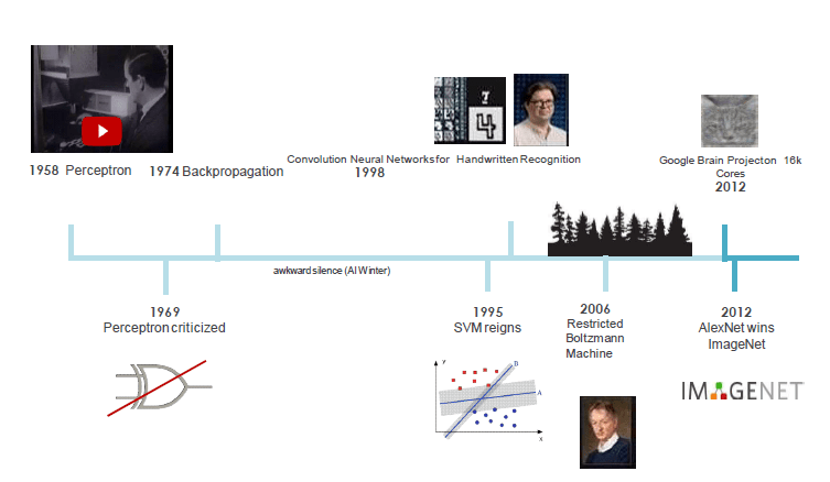
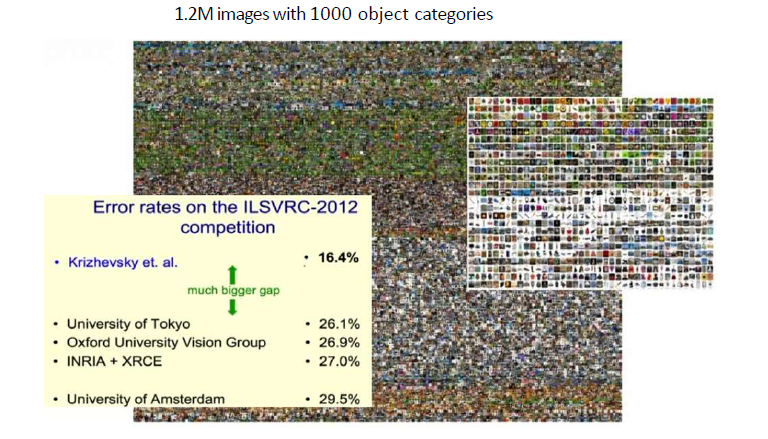
ImageNet Challenge 2012
Why second wave?
- With the advancement in Internet of Things IoT, More data from systems and sensors
- More compute power : GPU’s, multi-core CPU’s
- Training of Deep Architectures become faster
- With more data in place, data driven decisions are in demand than to only rely on experience driven decisions

Machine learning vs Deep learning

As it is very clear from the above image that, in Machine Learning, one has to program for feature extraction and then pass those feature to the models for classification or prediction. And hence these two steps happen independently. However, with the large amount of data it becomes near to impossible to extract features correctly and then pass them to the model for classification. Hence deep learning approach takes the advantage of high computation power which is available now a days, and takes huge raw data which further processed among different deep layers. And then the last layer which is called as output layer ultimately gives the classification results. So you see feature extraction and classification both happen within the deep layers.
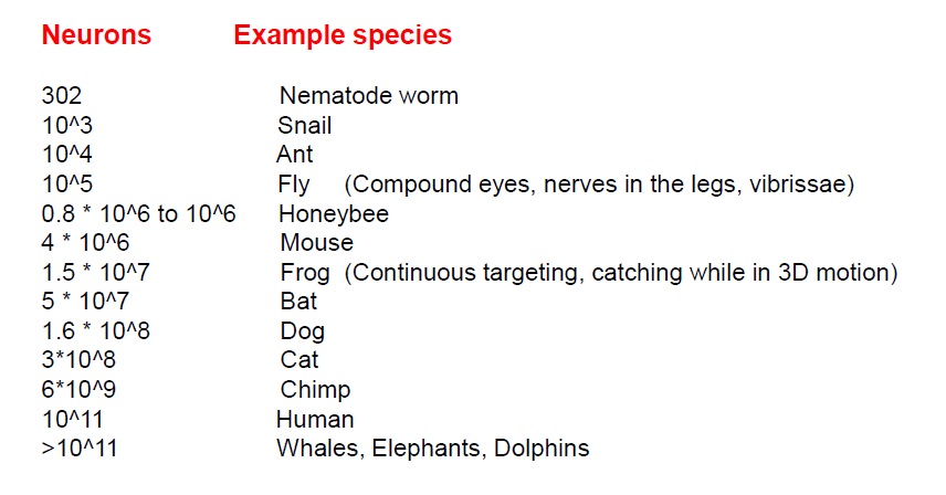
Thinking is possible even with a “small” brain
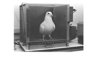


Results of above Experiments
- Pigeons were able to discriminate between Van Gogh and Chagall with 95% accuracy (when presented with pictures they had been trained on)
- Discrimination still 85% successful for previously unseen paintings of the artists
- Mice can memorize mazes, odors of contraband (drugs / chemicals / explosives)
Applications of ANN/DL
- Finance domain (Categorical and Numerical data) :
- Identify the fraud detection in credit card transactions
- Healthcare domain (Image data):
- Lung cancer classification of images / TB detection from chest images
- Social media(Image data):
- Face recognition and tag the people
- Across the domains (Text):
- Identify the potential cases of automation from historical ticket data
- Build a chat bot
Image Segmentation
Identification of different objects in the image.
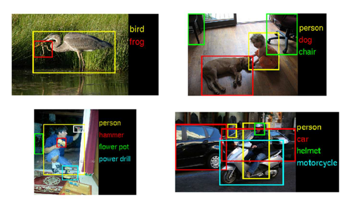
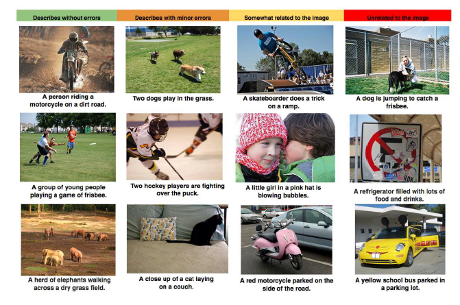
Image annotation
Annotate what is happening in the image. something like labeling the image with the best described label.
Video Classification
Identify what the video all about. for example what kind of sport is is being played in the video.

–Andrej Karpathy (Google/Stanford)
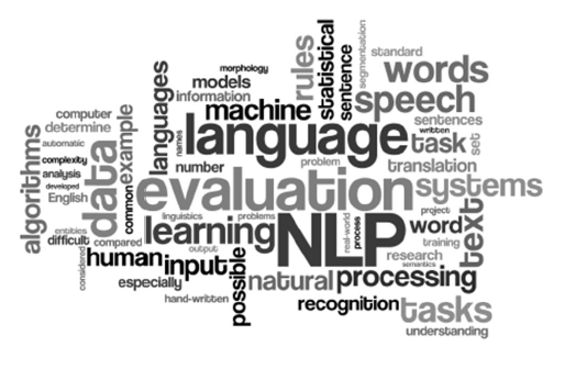
Natural language processing
Process the raw text to extract important information.
- semantic parsing
- search query retrieval
- sentence modeling
- classification
- prediction
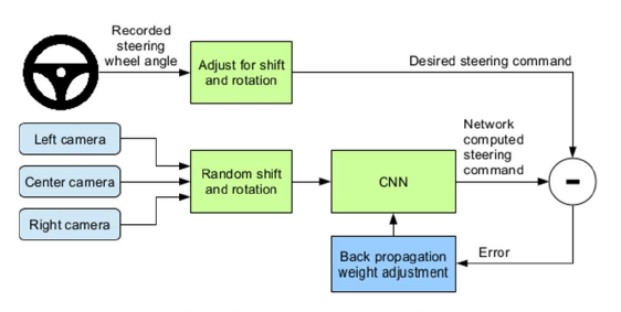
Autonomous driving
Once trained, the network can generate steering commands from the video images of a single center camera.

Corporation]
So, how does the brain work?
Direction of signal is along the Axon from Nucleus to synapse

Biological neural networks

- Fundamental units are termed neurons.
- Connections between neurons are synapses.
- Adult human brain consists of 100 billion neurons and 1000 trillion synaptic connections.
- Equivalent to computer with one trillion bit per second processor
Neurons in various species
Artificial neural network
Activation function plays an important role in classifying the objects in different categories.

Fundamentals

DL is a class of ML algorithms use a cascade of many layers of nonlinear processing units for
feature extraction and transformation.
A neural net model is composed a set of Layers. There are many types of layers available and each layer has many parameters. Thus we can have infinitely many different network architectures.
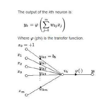
Artificial neural network
Artificial neurons are elementary units in an artificial neural network. The artificial neuron receives one or more inputs (representing dendrites) and sums them to produce an output (or
activation) (representing a neuron’s axon).
Usually the sums of each node are weighted, and the sum is passed through a non-linear function known as an activation function.
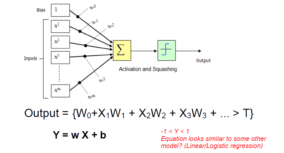
Artificial neural model: Perceptron
Learning process
General Training Steps
- Learning is changing weights
- In the very simple cases
- Start random
- If the output is correct then do nothing.
- If the output is too high, decrease the weights attached to high inputs
- If the output is too low, increase the weights attached to high inputs
Feed forward nets
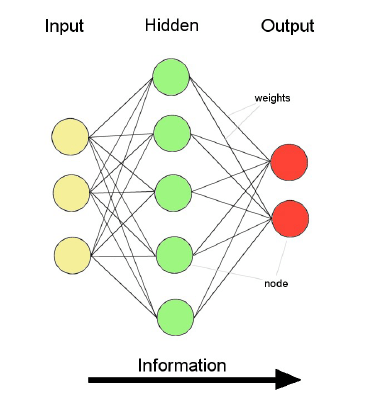
- Information flow is unidirectional
- Data is presented to Input layer
- Passed on to Hidden Layer
- Passed on to Output layer
- Information is distributed
- Information processing is parallel
- Back propagation
- Requires training set (input / output pairs)
- Starts with small random weights
- Error is used to adjust weights (supervised learning)
What are hidden layers?
They are non-linear sums of the inputs
So, they are not linearly dependent on inputs (they are non-linearly dependent)
They are engineered features of the original inputs!
- Feature engineering is so difficult because for each type of data and each type of problem, different features do well
- Neural networks can potentially build features hierarchically
But, how to learn hidden weights

Back propagation
With the concept of gradient descent
- Forward propagation: Activation [input * weight matrix]
- To get optimal value of each weight:
- Direction is opp. to the gradient
- Find weight with minimum error
- Derivative (slope of a tangent line – rate of change of a function)
- Partial derivative (w.r.t. one of the variables)
- Chain rule (derivatives of composite functions)
- calculate the error w.r.t. each weight
- New weight = old weight – Derivative Rate * learning rate
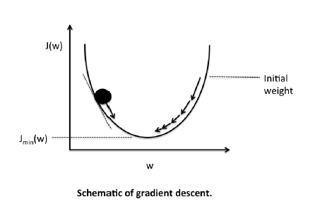
Gradient descent
- Randomly start somewhere and compute slope using calculus.
- Update the coefficients in the negative slope direction
- Repeat until convergence
- Gradient descent is greedy
- Multiple initiations and selection of the best is the option
- No way to theoretically guarantee convergence to global optimum.
- But, generally convergence to a local optimum which is very close to global.
- Therefore state-of-the-art results 🙂
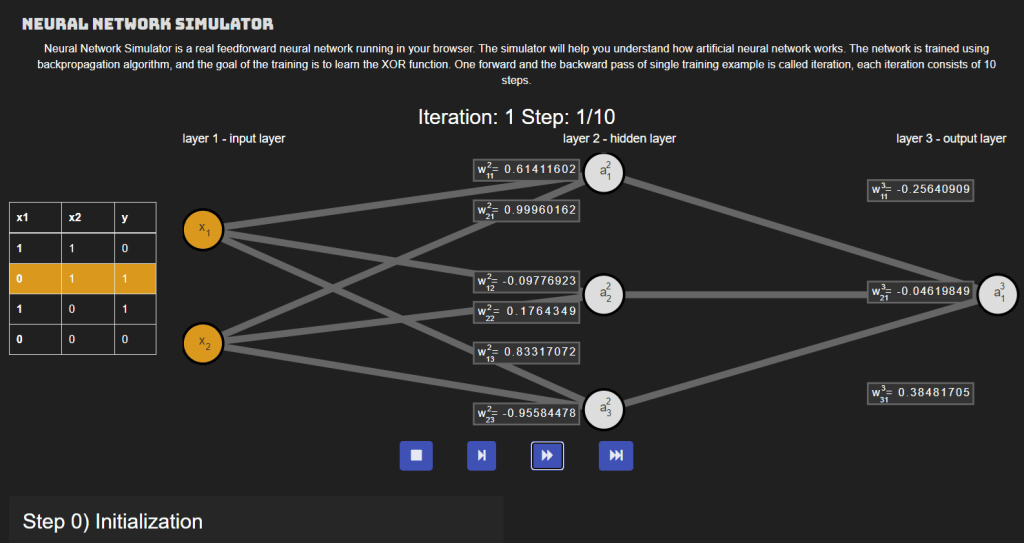
Neural Network simulator
Please refer the link https://www.mladdict.com/neural-network-simulator for the live visualization and understanding by doing.
Activation Functions
In Neural Networks, the activation function of a node defines the output of that node given an
input or set of inputs.
A standard computer chip circuit can be seen as a digital network of activation functions that
can be “ON” (1) or “OFF” (0), depending on input.
This is similar to the behavior of the linear perceptron in neural networks.
It is the nonlinear activation function that allows such networks to compute nontrivial problems
using only a small number of nodes.
ReLu: max(0,x)
Properties of activation function
Nonlinear:
When the activation function is non-linear, then a two-layer neural network can be proven to be a universal function approximator.
Continuously differentiable:
This property is necessary for enabling gradient-based optimization methods.
Range:
- When the range of the activation function is finite, gradient-based training methods tend to be more stable.
- Smaller learning rates are typically necessary.
Monotonic:
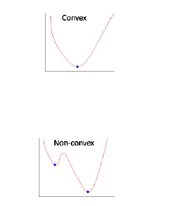
When the activation function is monotonic, the error surface associated with a single-layer model is guaranteed to be convex.
Smooth
Functions with a Monotonic derivative have been shown to generalize better in some cases.
Approximates identity near the origin:
- The neural network will learn efficiently when its weights are initialized with small random values.
- When the activation function does not approximate identity near the origin, special care must be used when initializing the weights.

Different Layers
- Dense Layer
- Dropout Layer
- Convolution1D
- Convolution2D
- MaxPooling1D
- LSTM
Will explain the working of each layer in detail in next article.
Parameters to vary for Model Tuning
- Number of layers
- Number of neurons in each layer
- Activation function in each layer
- Number of epochs
- Error/loss functions
- Iteration (equivalent to when a weight update is done)
- Learning rate (α)
- Size of the step in the direction of the negative gradient
- Batch size
- Momentum parameter (weightage given to earlier steps taken in the process of gradient descent)
- Kernels
- Number of features
- Number of filters for images
- Filter sizes for images
- Gradient descent methods
Recap of evaluation measures

Precision: When it predicts yes, how often is it correct?
TP/predicted yes = 100/110 = 0.91
“Sensitivity” or “Recall”: When it’s actually yes, how often does it predict yes?
TP/actual yes = 100/105 = 0.95
Accuracy: Overall, how often is the classifier correct?
(TP+TN)/total = (100+50)/165 = 0.91
Misclassification Rate: Overall, how often is it wrong?
(FP+FN)/total = (10+5)/165 = 0.09
equivalent to 1 minus Accuracy also known as “Error Rate”
False Positive Rate: When it’s actually no, how often does it predict yes?
FP/actual no = 10/60 = 0.17
Specificity: When it’s actually no, how often does it predict no?
TN/actual no = 50/60 = 0.83
equivalent to 1 minus False Positive Rate
This is all about basics of Artificial Neural Networks. In my upcoming posts I will be writing in detail about each topics mentioned in this post. So stay tuned!!!
Thank you.

One comment