In this post I have put together the practice problems (from my academics study notes) to explain how in practical Hypothesis Testing works. This post is written mostly for the learners who want to deep dive into the statistics for data science. Focus will be on problem solving. For concepts please refer my previous posts on testing of hypothesis.
Prerequisite to understand Hypothesis testing examples:
- Understanding of hypothesis testing concepts
- How to use z-table, t-table and chi square table.
Formula list:
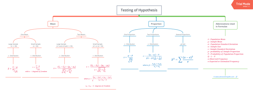
Critical Regions
In hypothesis testing, critical region is represented by set of values, where null hypothesis is rejected. So it is also know as region of rejection. It takes different boundary values for different level of significance. Below info graphics shows the region of rejection that is critical region and region of acceptance with respect to the level of significance 1%.
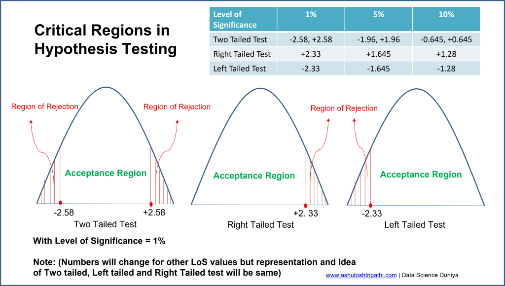
| LoS -> | α = 1% | α = 5% | α = 10% |
|---|---|---|---|
| Two Tailed Test | (-2.58, +2.58) | (-1.96, +1.96) | (-0.645, +0.645) |
| Right Tailed Test | +2.33 | +1.645 | +1.28 |
| Left Tailed Test | -2.33 | -1.645 | -1.28 |
Question 1
A Telecom service provider claims that individual customers pay on an average 400 rs. per month with standard deviation of 25 rs. A random sample of 50 customers bills during a given month is taken with a mean of 250 and standard deviation of 15. What to say with respect to the claim made by the service provider?
Solution:
First thing first, Note down what is given in the question:

H0 (Null Hypothesis) : μ = 400
H1 (Alternate Hypothesis): μ ≠ 400 (Not equal means either μ > 400 or μ < 400 Hence it will be validated with two tailed test )
σ = 25 (Population Standard Deviation)

LoS (α) = 5% (Take 5% if not given in question)

n = 50 (Sample size)
xbar x̄ = 250 (Sample mean)
s = 15 (sample Standard deviation)

n > = 30 hence will go with z-test

Step 1:
Calculate z using z-test formula as below:

z = (x̄  - μ)/ (σ/√n)
z = (250 - 400) / (25/√50)
z = -42.42

Step 2:
get z critical value from z table for α = 5%
z critical values = (-1.96, +1.96)
to accept the claim (significantly), calculated z should be in between
-1.96 < z < +1.96

but calculated z (-42.42) < -1.96 which mean reject the null hypothesis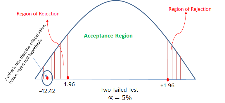
Question 2
From the data available, it is observed that 400 out of 850 customers purchased the groceries online. Can we say that most of the customers are moving towards online shopping even for groceries?
Solution:

Note down what is given:
400 out of 850 which indicates that this is a proportion problem.

Proportion p (small p) = 400/850 = 0.47

H0 (Null Hypothesis): P (capital P) > 0.5 (claim is that most of the customers are moving towards online shopping even for groceries which mean at least 50% should do online shopping)
H1 (Alternate Hypothesis): P < = 0.5 left tailed

n = 850
LoS (α) = 5% (assume 5% as it not given in question)

n > = 30 hence will go with z-test

Step 1:
calculate z value using the z-test formula
z = (p - P)/√(P*Q/n)
z = (0.47 - 0.50)/√(0.5*0.5/850)
z = -1.74

Step 2:
get z value from z table for α = 5%
From z-table, for α = 5%, z = -1.645 (one value as it is one (left) tailed problem)
z(calculated) -1.74 < -1.645 (z from z-table with α = 5%)

Conclusion:
Hence we reject the null hypothesis that mean, with given data we can validate significantly that most of the customers are not moving towards online shopping even for groceries.
Question 3
It is found that 250 errors in the randomly selected 1000 lines of code from Team A and 300 errors in 800 lines of code from Team B. Can we assume that team B’s performance is superior to that of A.
Solution:

Note down what is given in the question:

There are two samples : Team A and Team B
for each Team some proportion is given in terms of line of error out of total line of code.
Hence this problem can be solved using two proportion z-test.

For one or two proportion type problem we use z-test. (in case of multi-proportion we use χ2 that is chi square test)

Team A (Sample A):
proportion pA (small p) = 250/1000 = 0.25
nA = 1000

Team B (Sample B):
proportion pB (small p) = 300/800 = 0.375
nB = 800

Take α = 5% (assume α = 5% if not given in question)

Claim: Team B's performance is superior than Team A which means:
H0 (Null Hypothesis): overall mean error of Team B  μB < μA overall mean error of Team A (with respect to population)
H1 (Alternate Hypothesis) : μB > = μA (one right tailed test)

Step 1:
calculate z value from two proportion z-test formula as below:

z = (pA - pB)/sqrt([p^(1-p^)(1/nA + 1/nB)])
where p^ (p hat) = (nA*pA + nB*pB)/(nA + nB)

p^ (p hat) = (1000*0.25 + 800*0.375) / (1000 + 800) = 0.305

z = (0.25 - 0.375) / sqrt([0.305*(1-0.305)*(1/1000 + 1/800))
z = -0.125/[0.02185]
z = -5.72

Step 2:

get z using z-table for α = 5% which is z = +1.645

Now calculated z -5.72 < +1.645

Hence will conclude that null hypothesis is true which mean from given data it is proven significantly that team B's performance is better that team A's performance.
Question 4
Following is the record of number of accidents took place during the various days of the week.
| Monday | Tuesday | Wednesday | Thursday | Friday | Saturday | Sunday |
|---|---|---|---|---|---|---|
| 120 | 140 | 200 | 90 | 140 | 120 | 180 |
Can we conclude that accident s are independent of the day of week?
Solution:
H0 (Null Hypothesis): Accidents are independent of the day
H1 (Alternate Hypothesis): Not independent

Here each day will represent a sample and observed accident data is proportion.
Hence this problem can be categorized as multi proportion problem and will be solved using χ2 chi square test.
Below table shows the Observed values of accident in first column
As we want to validate that accidents are independent of the day of week.

for that average accidents on each day should be different. Hence we need to calculate average accidents on each day and this will be called as expected value in χ2 test.

Take α = 5% (assume α = 5% if not given in question)

Step 1: calculate expected values and χ2 values using χ2 formula as shown below in the table| Observed (o) | Expected (e = average of Observed values) e = (990/7) | χ2 = Σ[(o-e)2]/e |
|---|---|---|
| 120 | 141.43 | 3.11 |
| 140 | 141.43 | 0.01 |
| 200 | 141.43 | 27.91 |
| 90 | 141.43 | 18.03 |
| 140 | 141.43 | 0.01 |
| 120 | 141.43 | 3.11 |
| 180 | 141.43 | 10.87 |
| Total = 990 | Total χ2 = 63.05 |
Step 2: use χ2 table for α = 5% and get χ2 value from the table.
from table we got χ2 (critical value at α = 5%) = 3.841

Step 3: compare both χ2  values.

The chi-square value of 63.05 is much larger than the critical value of 3.84, so
the null hypothesis can be rejected.

It means, reject the null hypothesis and accept the alternate hypothesis. Which means with given data we can conclude significantly that accidents are not independent of the day of week. [might not look realistic but with given data is concluding this]
Question 5
Analyze the below data and tell whether you can conclude that smoking causes cancer or not?
| Category | Diagnosed as Cancer | Without Cancer | Total |
|---|---|---|---|
| Smokers | 400 | 300 | 700 |
| Non-Smokers | 300 | 500 | 800 |
| Total | 700 | 800 | 1500 |
chi square test check the independence of the two categorical variable. Here in this question we need to test whether smoking and cancer are independent or dependent to each other. Hence will perform chi square test.

Solution:

Step 1:
H0 (Null Hypothesis): Cancer is dependent on smoking
H1 (Alternate Hypothesis): cancer is not dependent on smoking

Step 2:
Calculate the expected value for each cell of the table (when null hypothesis is true)
The expected values specify what the values of each cell of the table would
be if there is no association between the two variables.

The formula for computing the expected values requires the sample size, the
row totals, and the column totals.

expected value (e) = (row total * column total)/table total

Now lets create another table with observed and expected values both:| Category | Diagnosed as Cancer | Without Cancer | Total |
|---|---|---|---|
| Smokers | o = 400, e = 700*700/1500 = 326 | o = 300, e = 700*800/1500 = 373 | 700 |
| Non-Smokers | o = 300, e = 800*700/1500 = 373 | o = 500, e = 800*800/1500 = 426 | 800 |
| Total | 700 | 800 | 1500 |
Step 3:
calculate the chi square value:

                                   χ2 = Σ[(o-e)2]/e
χ2 = (400-326)2/326 + (300-373)2/373 + (300-373)2/373 + (500-426)2/426
χ2 = 16.79 + 14.28 + 14.28 + 12.85
χ2 = 58.2

Step 4:
Decide if χ2 is statistically significant.

The final step of the chi-square test of significance is to determine if the value
of the chi-square test statistic is large enough to reject the null hypothesis.

Now will check χ2 table for the critical value with α = 5%
So from table we got χ2 (critical value at α = 5%) = 3.841

The chi-square value of 58.2 is much larger than the critical value of 3.84, so
the null hypothesis can be rejected.

Which means with given data, it can be significantly concluded that cancer is not dependent on smoking.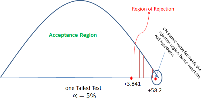
Question 6
It is claimed that the mean of the population is 67 at 5% level of significance. Mean obtained from a random sample of size 100 is 64 with SD 3. Validate the claim.
Solution:
First thing first, Note down what is given in the question:

H0 (Null Hypothesis) : μ = 67
H1 (Alternate Hypothesis): μ ≠ 67 (Not equal to means either μ > 67 or μ < 67 Hence it will be validated with two tailed test )

LoS (α) = 5%

n = 100 (Sample size)
xbar x̄ = 64 (Sample mean)
s = 3 (sample Standard deviation)

n > = 30 hence will go with z-test

Step 1: Calculate z using z-test formula as below:

z = (x̄  - μ)/ (σ/√n)
z = (64 - 67) / (3/√100) (in question population standard deviation is not given, in that case take sample standard deviation)
z = -10

step 2:

calculate z critical value for α = 5% from z-table.
so from z-table Z critical value = -1.96, +1.96 (will get two values due two tailed test)

step 3:

check if calculated z value is in between z critical value then accept the null hypothesis if z calculated is outside z critical then reject the null hypothesis.

Here, z calculated value = -10 which is much lesser than the left side z critical value -1.96, hence will reject the null hypothesis.

Conclusion:
with given data it is significantly proven that population mean is not equal to 67.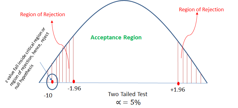
Question 7
There is an assumption that there is no significant difference between boys and girls with respect to intelligence. Tests are conducted on two groups and the following are the observations
| Mean | Standard Deviation | Size | |
|---|---|---|---|
| Girls | 75 | 8 | 60 |
| Boys | 73 | 10 | 100 |
Validate the claim with 5% LoS (Level of Significance)
Solution:
First thing first, Note down what is given in the question:

H0 (Null Hypothesis) : No difference between boys and girls in terms of intelligence. (μ2 = μ2)
H1 (Alternate Hypothesis): Boys and girls are different in terms of intelligence (μ2 ≠ μ2) => two tailed test

x1bar = 75 (boys sample mean)
x2bar = 73 (girls sample mean)
LoS (α) = 5%

In question, we have two sample mean. Boys sample mean and girls sample mean. Hence this can be solved with two mean problem.

Next both samples size n1 = 60 and n2 = 100 are greater than 30 hence will use z-test.

Step 1:
calculate z value from the two mean z test formula as below:

z = [(x1bar - x2bar) - (μ2 - μ2)]/√(s12/n1 + s22/n2)

μ2 - μ2 = 0 assuming null hypothesis is true

z = (75-73)/√(82/60 + 102/100)
z = 1.39

step 2:

calculate z critical value for α = 5% from z-table.
so from z-table Z critical value = -1.96, +1.96 (will get two values due two tailed test)

step 3:

check if calculated z value is in between z critical value then accept the null hypothesis if z calculated is outside z critical then reject the null hypothesis.

Here, z calculated value is in between the z critical values. -1.96 < 1.39 < 1.96
Hence will accept the null hypothesis.
Conclusion:
with given data it is significantly proven that there is no significant difference between the intelligence of boys and girls.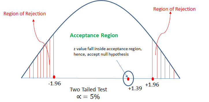
Question 8
An automobile tyre manufacturer claims that the average life of a particular grade of tyre is more than 20,000 km. A random sample of 16 tyres is having mean 22,000 km with a standard deviation of 5000 km.
Validate the claim of the manufacturer at 5% LoS.
Solution:
First thing first, Note down what is given in the question:

H0 (Null Hypothesis) : μ > 20000
H1 (Alternate Hypothesis): μ <= 22000 (less than mean one tailed test)


LoS (α) = 5% (Take 5% if not given in question)

n = 16 (Sample size)
x̄ = 22000 (Sample mean)
s = 5000 (sample Standard deviation)

n < 30 hence will go with t-test

step 1:

calculate t value from the t-test formula:
t = (x̄  - μ)/ (s/√n)
t = (22000 - 20000) / 5000/√16
t = 1.60

step 2:

get t critical value from t-table for α = 5% and degree of freedom = 16-1 = 15.
t critical value = 1.753

step 3:

check if t calculate < t critical then accept the null hypothesis else reject the null hypothesis.

Here, t calculated 1.60 < t critical 1.753, hence will accept the null hypothesis.

Conclusion:

from the data given, it is significantly proven that average life of the tyres is more than 20000.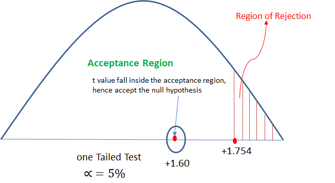
That is all for now. Please share your thoughts using the comment section below.

I have a doubt about Question-8. From what I’ve been taught the null hypothesis always has to have the equal sign. So according to that, the first step for Q8 would be null hypothesis : μ<= 20,000 and the alternate hypothesis μ> 20,000. Then, this becomes a right tailed test. We continue the calculations and everything and we get tα= 1.753 and we get t = 1.6. Since t= 1.6<1.753 H₀ is not rejected. BUT my H₀ is μ<= 20,000 which means we have enough evidence to support that the average life of the tyres is less than or equal 20000. OR it is not more than 20,000.
LikeLike
Solution to question #2 is wrong because the value of Step 1: calculate z value using the z-test formula z = (p – P)/√(P*Q/n) z = (0.47 – 0.50)/√(0.5*0.5/850) z = 1.74 should be negative value. So in the conclusion you should be comparing -1.64 vs -1.74 and since -1.74 falls under the rejection region, you should be rejecting the null hypnosis
LikeLiked by 1 person
Thank you Karan. solution is updated.
LikeLiked by 1 person
I think smoking problem is wrongly concluded. There the H0 is assumed of dependency(smoking and cancer are dependent) while for chi square test, the null hypothesis is always for independence. So the H0 should be “Smoking and Cancer are independent”.
LikeLiked by 1 person
Please how can I download this page?
LikeLiked by 1 person
In the last sum the alternate hypothesis is less than 22,000 and the null hypothesis is more than 20,000. If the value turns out to be 21,000 then which hypothesis will you accept? I guess there’s an error, the alternate hypothesis should be less than equal to 20,000 and not 22,000. Correct me if I’m wrong.
LikeLiked by 1 person
Hi,
Thanks for presenting above test cases, it really really helps to understand the tail concept. I am reading z-test and refer your hypothesis page as an example. I go through z-test example and in example no.8 last one it is “One tail – Left tailed test” but in the diag below it shows the right tailed. Not sure am I interpret wrong or diag error ? pls . correct me. Thanks.
LikeLiked by 1 person
The alternate hypothesis is the opposite of null hypothesis so it’s less less than or left tailed. Since the null hypothesis was accepted the graph is Right Tailed had the null hypothesis been rejected or the alternate hypothesis been accepted the graph would have been left tailed. I hope I cleared your doubt
LikeLiked by 1 person