Decision Tree is one of the easiest algorithm to understand and interpret. If you are familiar with if-else statements in programming then that is pretty much all you need to know to understand how decision tree algorithm works. Even if you are not familiar with programming then also if you apply your common sense and relate with the real life examples, then you will easily understand the decision tree algorithm. For example if vehicle has fuel then it will start, if you try then you can fail or succeed, if it is rainy, match will not happen etc… So based on these conditional statement only decision tree helps us to build a model to predict something for future.
Decision Tree is supervised machine learning algorithm which is used for both types of problems regression (that is predicting the continuous value for future example house price, hours the match can be played given overcast condition etc…) and classification (that is classifying different objects into respective categories or classes for example given the overcast conditions match will be played or not, given image belongs to cat or dog etc…).
Table of Content
- Important Definitions
- Different Nodes in Decision Tree
- Different Algorithms used to build Decision Tree
- Decision Tree for Classification
- Decision Tree for Regression
Important Definitions
Homogeneous and Heterogeneous Data Nodes
Understanding homogeneous nature of data nodes is very important when it comes to decision tree. It is directly related to the predictive power of the tree build. If you pick a random data item from a fully homogeneous node then it wont be any brainier for you to tell which class it belongs to. Got the idea? if not then let me explain what is meant by homogeneous and non homogeneous data nodes.
A fully homogeneous node is one which has all the data items belonging to the same class. And as we keep on mixing the data items from different classes it becomes a non homogeneous or heterogeneous node. So a fully heterogeneous data node will be the one which has equal proportion of all classes data items. Lets understand the same by visualizing some plots as below:

Above pic is self explanatory, still i want to emphasize one thing that how mathematically you will measure the level of homogeneity in a node? Because this level of homogeneity helps you to decide on where to split the data and how to form the decision tree. That is where concepts of Entropy, Information Gain and Gini Impurity comes in picture.
Entropy and information Gain
Entropy is the measure of randomness in your data. More randomness means more entropy means harder to draw any conclusion or harder to classify. Lets relate it to the homogeneity concept explained above to make it easy to understand. If your data node is heterogeneous it will be hard to draw any conclusion about that data node which will lead to higher entropy.
High Entropy Means More Randomness means less Homogeneous (Heterogeneous)
If the sample or data node is completely homogeneous, Entropy = 0
If the sample or data node is equally divided among classes, Entropy = 1
So in decision tree each split is based on reduction in entropy so that we can reach towards the less heterogeneous or more homogeneous node. So we split in such a way that after every split we get more homogeneous node so that drawing conclusion becomes easy. And hence in each split there will be reduction in entropy. And this reduction in entropy is known as Information gain.

in the above plot, it is visible that when we have the perfect outcome which mean probability value equal to either 1 or 0 then Entropy is 0. Mean there is no randomness involved. And when degree of randomness increases probability will be mapped in between 0 to 1. For probability = 0.5 (both events are equally likely) there will be maximum randomness and hence Entropy will be maximum that is 1.

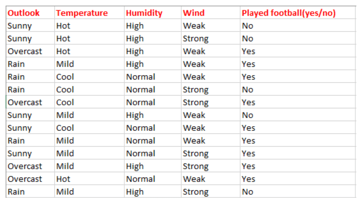
We will be using below data for calculation purpose (Even for the next definitions in the post)
Entropy Calculation
Entropy of Target Variable
Entropy for target variable (Play Football Yes/No). First of all we need to group data based on the classes in target variables.
Play Football
| Yes | No |
|---|---|
| 9 | 5 |
Entropy(Play Football) = ?
Here there are two classes yes and no so need to calculate probability of each class.
P(Yes) = count where play is yes/ total count of rows = 9/14,
Similarly P(No) = 5/14
Now using the formula of Entropy H(play) will be

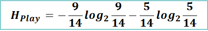
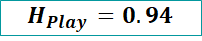
This entropy of play is with respect to the complete data.
Now in decision tree, we need to decide which node will be the root node and which one will be subsequent nodes. So we calculate entropy of target with respect to each independent variable and see where we get least entropy mean least randomness. mean most homogeneity. And that will be the node which will produce even more homogeneous data after split. This node will become the root node. and then process will be repeated for the subsequent nodes. Hence we should know how to calculate entropy with respect to other independent variables.
Entropy of target with respect to independent variable.
Example Calculate Entropy of target with respect to Outlook. (Note: This will be used in deciding on which node or column to split the tree. This concept I will explain in more detail in next sections under decision tree building using entropy)
| Outlook | Yes | No | Total |
|---|---|---|---|
| Rainy | 3 | 2 | 5 |
| Overcast | 4 | 0 | 4 |
| Sunny | 2 | 3 | 5 |
| 14 |
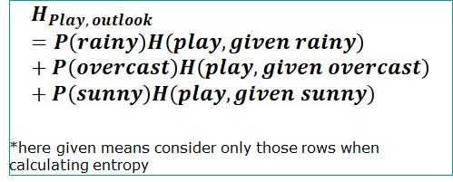
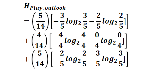
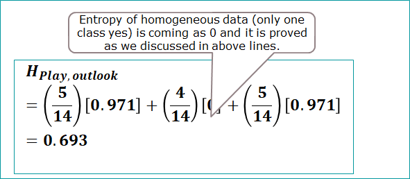
Now to calculate Entropy(Play, given Outlook), will calculate weighted entropy of play individually for rainy, overcast and sunny and then sum them all.
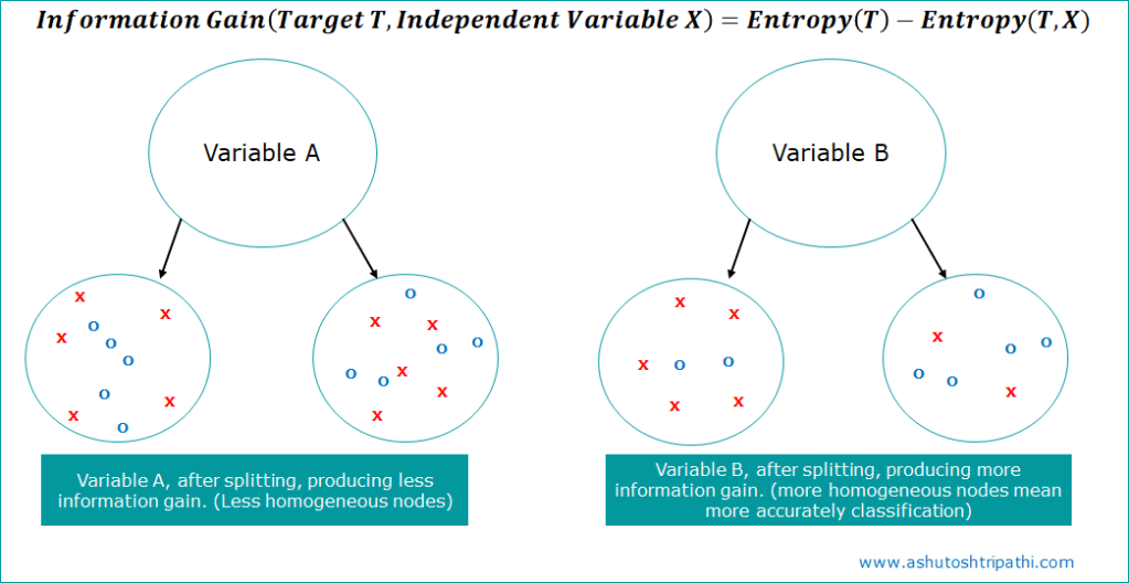
Information Gain
Information gain is the measure of homogeneity we achieve after splitting a data node. In statistical terminology the amount of reduction in entropy after splitting the data node is known as information gain.

From above formula you can easily say that:
More Information Gain = Less Entropy(T,X) = More Homogeneous Node
This goes in align with our objective of getting the more homogeneous data node after the split. So we calculate the entropy of target with each independent variable and see where information gain is more means where we getting more homogeneous node. So the variable which has more information gain will be placed at root.

Suppose a dataset contains two variables which mean two nodes. And in below image i tried to visualize that how splitting look like if we try to split by A and B separately. So if you see when we try to split with B then we get comparatively more homogeneous nodes. This means splitted nodes have more proportion of one class than the other class.
There is another criteria to split the node that is using Gini and Gini Impurity. Let’s understand more about Gini criteria.
Gini and Gini Impurity
Gini is calculated by using the formula – the sum of square of probability for success and failure (p^2+q^2)
Gini is directly proportional to homogeneity. Higher the value of gini higher the level of homogeneity after the split.
Gini Impurity is inversely proportional to the homogeneity. So while spliting we look for least gini impurity and the node which has least gini impurity is made as root node.

Classification and Regression Tree (CART) algorithm uses gini score as the criteria to split the nodes in decision tree. And other important point is that Gini works only for binary split with categorical target as success or failure.
Lets take the football play example data and calculate gini for the outlook column.
| Outlook | Play Football (Yes) | Play Football (No) | Total |
|---|---|---|---|
| Rainy | 3 | 2 | 5 |
| Overcast | 4 | 0 | 4 |
| Sunny | 2 | 3 | 5 |
| | | | 14 |
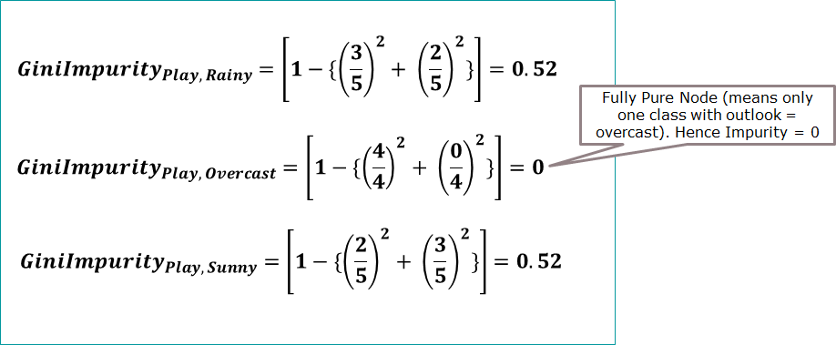
Here again similar to entropy of target with respect to independent variable, will calculate gini of target with respect to independent variable and it is also known as weighted gini.
Here also will calculate weighted gini with respect to rainy, overcast and sunny rows and sum them all to get the final gini value for outlook column.
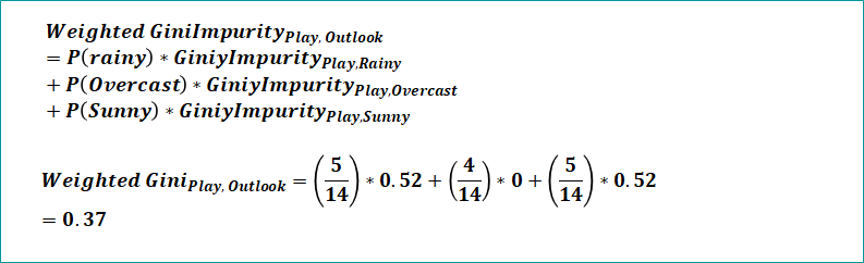
Similarly you can create the gini impurity for other independent variables and see which has least gini impurity. The one which has least gini impurity will be the root node.
Reduction in Variance or Standard Deviation Reduction – SDR
Entropy, Information Gain and Gini Impurity are used in classification problems. So what about regression? So similar to information gain that is reduction in entropy, we have reduction in variance or reduction in standard deviation which is used for regression type problem in decision tree.


So we calculate weighted SDR with respect to independent variable and see where we get more SDR value and that will be the root node.
| Outlook column values | Hours Played | Count |
|---|---|---|
| Standard Deviation for respective outlook condition | ||
| rainy | 10.87 | 5 |
| overcast | 3.49 | 4 |
| sunny | 7.78 | 5 |
To calculate standard deviation for individual attributes for example rainy outlook then consider only rainy rows data and apply the formula on hours played.


Standard Deviation Reduction is based on the decrease in standard deviation after the split. So the variable which gives highest SDR will be declared as the root node. And the highest SDR will corresponds to the most homogeneous nodes after the split.
Understand different nodes in Decision Trees

- Root Node: It represents the entire population or sample and this further gets divided into two or more homogeneous sets. If you consider Information gain then the node which has maximum information gain will become the root node.
- Decision Node: When a sub-node splits into further sub-nodes, then it is called the decision node. Basically it helps you to decide whether to choose (select or go) right sub tree or left sub tree
- Leaf / Terminal Node: Nodes do not split is called Leaf or Terminal node.
- Branch / Sub-Tree: A subsection of the entire tree is called branch or sub-tree.
- Parent and Child Node: A node, which is divided into sub-nodes is called a parent node of sub-nodes whereas sub-nodes are the child of a parent node.
- Pruning: When we remove sub-nodes of a decision node, this process is called pruning. You can say the opposite process of splitting. It is used in hyper parameter tuning in decision trees.
Different Algorithms used to build Decision Tree
Decision Tree is used for both types of problems Classification and Regression. So based on problem types it uses different algorithms.
Algorithms are also categorized based on the different splitting criteria like entropy, information gain, gini and gini index, and standard deviation reduction.
Let us look at some algorithms used in Decision Trees:
ID3 → (Iterative Dichotomiser 3, uses entropy and information for classification problems and standard deviation reduction for regression problems)
C4.5 → (successor of ID3 and used for classification)
CART → (Classification And Regression Tree. used for both classification and regression)
CHAID → (Chi-square automatic interaction detection Performs multi-level splits when computing classification trees)
MARS → (multivariate adaptive regression splines)
Decision Tree for Classification Problems
Building a decision tree for the given data using Entropy and Information
Please watch the video explaining decision tree formation and split using entropy and information gain.
Building a decision tree for the given data using Gini and Gini Index
Please watch the video which explains decision tree formation using gini and gini index.
Complete Code to build Decision Tree for classification using Python
Please refer my post on step by step guide to build decision tree using python.
Decision Tree for Regression
Please refer my post on step by step guide to build decision tree for Regression
