Numerical Feature Extraction from Text | NLP series | Part 6

Background

Machine Learning algorithms don’t understand the textual data rather it understand only numerical data. So the problem is how to convert the textual data to the numerical features and further pass these numerical features to the machine learning algorithms.

As we all know that the raw text stored in some dump repository contains a lot of meaningful information. And in today’s fast changing world, it becomes essential to consider data driven decision than fully rely on experience driven decision.

It even requires to analyse the live textual data. For example analysis of live user feedback, Analysing user browsing history to recommend the results based suited to individual’s need.

Other use cases could be Sentiment Analysis, Similarity matching between documents, Important Named Entity Recognition from the documents etc.

Key takeaways from this post:

• Understand what is Feature Extraction.
• Count Vectorizer
• Term Frequency
• Inverted Document Frequency
• tf-idf Vectorizer
• Pass these numerical features to the Machine Learning Algorithms
• Build a LinearSVC classifier to classify the spam text.

You may like to read the previous articles of NLP Series. Here are the links:

• SPACY INSTALLATION AND BASIC OPERATIONS | NLP TEXT PROCESSING LIBRARY | PART 1
• A QUICK GUIDE TO TOKENIZATION, LEMMATIZATION, STOP WORDS, AND PHRASE MATCHING USING SPACY | NLP | PART 2
• PARTS OF SPEECH TAGGING AND DEPENDENCY PARSING USING SPACY | NLP | PART 3
• NAMED ENTITY RECOGNITION NER USING SPACY | NLP | PART 4
• HOW TO PERFORM SENTENCE SEGMENTATION OR SENTENCE TOKENIZATION USING SPACY | NLP SERIES | PART 5

Methods to extract numerical features from Text

1. Count Vectorizer

Simply count the occurrence of each word in the document to map the text to a number.

While counting words is helpful, it is to keep in mind that longer documents will have higher average count values than shorter documents, even though they might talk about the same topics. Hence counting words is not enough to describe the features of the text.

To overcome this we have something called term frequency as the next method.

2. Term Frequency tf(t,d)

To avoid the shortcomings of count vectorizer, we can simply divide the number of occurrences of each word in a document by the total number of words in the document.

These new features are called tf – Term Frequencies.

Even term frquency tf(t,d) alone isn’t enough for the thorough feature analysis of the text. Let’s understand this with an example.

Consider the frequently occuring words like “is”, “am”, “are” .. “the”..etc.

In this case the term frequency method will tend to incorrectly emphasize the documents which happen to use the words like “the” more frequently. And it will give less weightage to the more meaningful words like “ecommerce”, “red”, “lion” etc. which might be occuring less frequently in the document compare to the word “the”.

These more frequently occuring words are known as STOP WORDS

Again we have something better than alone term frequency known as the tf-idfVectorizer which will understand in the next method.

3. tf-idf Vectorizer

Another refinement on top of tf is to downscale weights for words that occur in many documents in the corpus and are therefore less informative than those that occur only in a smaller portion of the corpus and are more informative.

This downscaling is called tf–idf for “Term Frequency times Inverse Document Frequency”.

Inverse Document Frequency idf: It is the logarthmically scalled inverse fraction of the documents that contains the term.

It is obtained by dividing the total no of documents by the number of documents containing the term and then taking the logarithm of that quotient.

So the Inverse Document Frequency factor reduces the weight of the terms which occur very frequently in many documents and increases he weight of the terms which occur rarely or in few documents.

Note:

tf-idfVectorizer is the combination of CountVectorizer, tf and idf factors.

just to make it more clear, we calculate the numerical feature for each unique word (called as term) in the document. And it generate the sparsh matrix of numerical features. Where header represents the unique terms and row index represent the different documents.

There is is one more method called word2vec which is also used for feature extraction, however that is more related with similarity matching. So I will be explaining this in detail in my next post.

With all these concept building lets start realizing them with the help of a data set.

import numpy as np
import pandas as pd

df = pd.read_csv('smsspamcollection.tsv', sep='\t')
df.head()

Note: Our objective is to understand the feature extraction, so not going in details of pre-processing steps. I will include all the steps in one complete end to end classification project which is my next post.

from sklearn.model_selection import train_test_split
X = df['message'] # this time we want to look at the text
y = df['label']
X_train, X_test, y_train, y_test = train_test_split(X, y, test_size=0.33, random_state=42)

Step 1. CountVectorizer

from sklearn.feature_extraction.text import CountVectorizer
count_vect = CountVectorizer()
X_train_counts = count_vect.fit_transform(X_train)
X_train_counts.shape

This shows that our training set is comprised of 3733 documents, and 7082 features.

Below is how 2D countVectorizer features look like.

print(X_train_counts)

Step 2. Transform Counts to Frequencies with Tf-idf

from sklearn.feature_extraction.text import TfidfTransformer
tfidf_transformer = TfidfTransformer()
X_train_tfidf = tfidf_transformer.fit_transform(X_train_counts)
X_train_tfidf.shape

Note: the fit_transform() method actually performs two operations: it fits an estimator to the data and then transforms our count-matrix to a tf-idf representation.

Alternatively Combine the Steps with TfidVectorizer

Actually we are combining the above two steps 1. Count Vectorizer which give the term count and 2. tf-idf which gives the term frequency and inverted document frequency in the single step with the help of TfidfVectorizer

from sklearn.feature_extraction.text import TfidfVectorizer
vectorizer = TfidfVectorizer()
X_train_tfidf = vectorizer.fit_transform(X_train) # remember to use the original X_train set
X_train_tfidf.shape

print(X_train_tfidf) # this return the same output as we got in step 2. sequence might be changed.

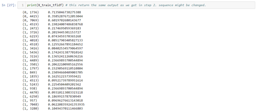
Above are the extracted Numerical Features from the raw text. Now these features can be passed directly to the Machine Learning algorithms as below.

Train a Classifier

Here we’ll introduce an SVM classifier. LinearSVC handles sparse input better, and scales well to large numbers of samples. The reason is our extracted numerical features are in sparse matrix form.

from sklearn.svm import LinearSVC
clf = LinearSVC()
clf.fit(X_train_tfidf,y_train)

Build a Pipeline

Remember that only our training set has been vectorized into a full vocabulary. In order to perform an analysis on our test set we’ll have to submit it to the same procedures. Fortunately scikit-learn offers a Pipeline class that behaves like a compound classifier.

from sklearn.pipeline import Pipeline
# from sklearn.feature_extraction.text import TfidfVectorizer
# from sklearn.svm import LinearSVC
text_clf = Pipeline([('tfidf', TfidfVectorizer()),
('clf', LinearSVC()),
])
# Feed the training data through the pipeline
text_clf.fit(X_train, y_train)

Test the classifier and display results

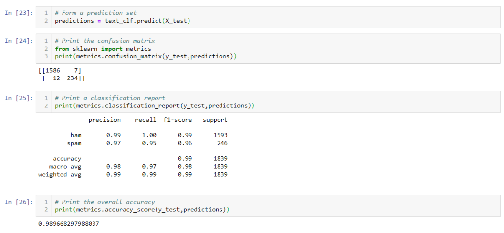
# Form a prediction set
predictions = text_clf.predict(X_test)

# Print the confusion matrix
from sklearn import metrics
print(metrics.confusion_matrix(y_test,predictions))

# Print a classification report
print(metrics.classification_report(y_test,predictions))

# Print the overall accuracy
print(metrics.accuracy_score(y_test,predictions))

So this is all about numerical feature extraction from text. I hope you like the article and it helps you to inhance your understanding on feature extraction techniques.

Next Article: Word2Vec and Semantic Similarity using spacy | NLP spacy Series | Part 7