A Step by Step Guide to Implement Decision Tree using Python | Machine Learning

In this we will learn from scratch how to implement decision tree using python. We will solve one classification problem and build the model from scratch. Following are the points we will be covering in this post:

Exploratory Data Analysis – EDA
Data Visualization
Data Pre-processing
Data Spliting- Stratified Sampling
Oversampling – SMOTE
Model Training
Fine Tuning
Hyper parameter Tuning

Problem Statement:

Predict whether a person will subscribe for the term deposit or not based on historical data given.

Virtual Environment Setup

#exceute below lines of code as command line to create a fresh virtual environment names "venvname"
python -m venv venvname
venvname\Scripts\activate
pip install jupyter
pip install ipykernel
ipython kernel install --user --name=venvname

Libraries Installation

#make sure you are inside the virtual environment as created in the above step.
#Now install the below libraries from command line
pip install pandas
pip install numpy
pip install matplotlib
pip install plotly
pip install seaborn
pip install sklearn
pip install pandas-profiling
pip install imblearn

Open Jupyter Notebook

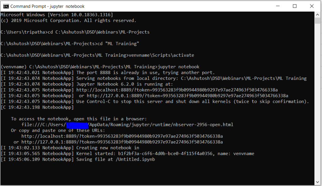
# now to open jupyet notebook type in command line
jupyter notebook #from inside the venvname

If you getting ther error like jupyter notebook not found even if you have done pip install jupyter then simply close the command prompt and reopen then go the path where you created the venvname and activate it. Now run the command “jupyter notebook” again it will open the jupyter.

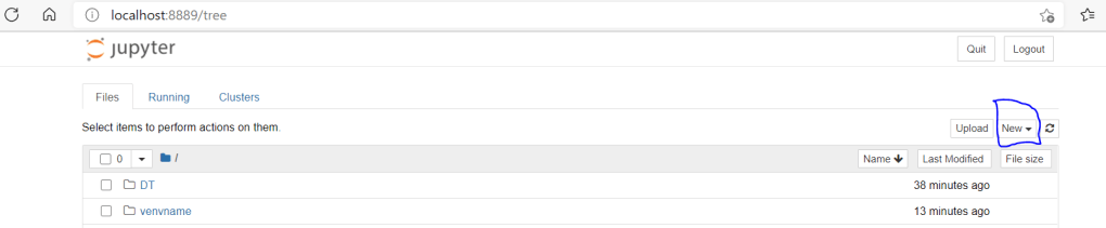
Now click on new button as highlighted in the above image. Here in drop down the newly created virtual environment will be shown as you have created the kernel for that already.

Select venvname, it will create an empty notebook in next tab. This is all about the setup. Now we will load the libraries and data set and learn the model building using decision tree classifier.

 
 import pandas as pd
 import numpy as np
 import matplotlib.pyplot as plt
 import seaborn as sns
 %matplotlib inline

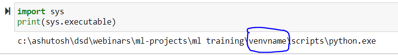
Validate if you are using the python interpreter from the virtual environment or not.

 
 import sys
 print(sys.executable)

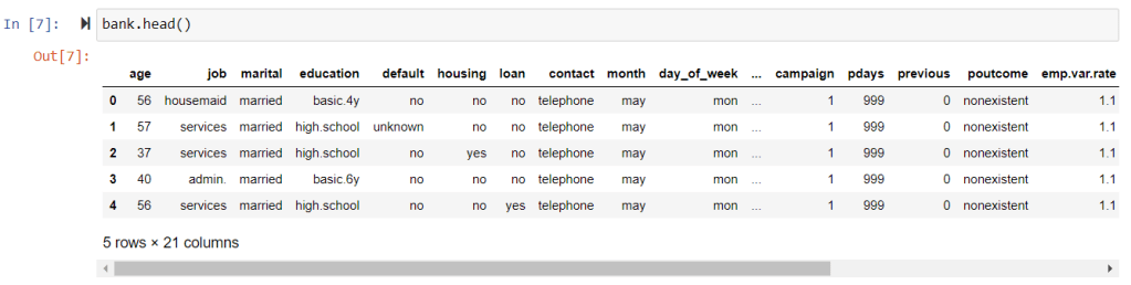
pd.read_csv("C:\Ashutosh\DSD\Webinars\ML-Projects\ML Training\DT\bank.csv",sep=";")

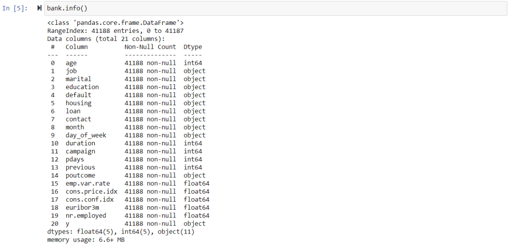
Features Description:

Bank client data:

age (numeric)
job : type of job (categorical: ‘admin.’,’blue-collar’,’entrepreneur’,’housemaid’,’management’,’retired’,’self-employed’,’services’,’student’,’technician’,’unemployed’,’unknown’)
marital : marital status (categorical: ‘divorced’,’married’,’single’,’unknown’; note: ‘divorced’ means divorced or widowed)
education (categorical: ‘basic.4y’,’basic.6y’,’basic.9y’,’high.school’,’illiterate’,’professional.course’,’university.degree’,’unknown’)
default: has credit in default? (categorical: ‘no’,’yes’,’unknown’)
housing: has housing loan? (categorical: ‘no’,’yes’,’unknown’)
loan: has personal loan? (categorical: ‘no’,’yes’,’unknown’)

8 – contact: contact communication type (categorical: ‘cellular’,’telephone’)

9 – month: last contact month of year (categorical: ‘jan’, ‘feb’, ‘mar’, …, ‘nov’, ‘dec’)

10 – day_of_week: last contact day of the week (categorical: ‘mon’,’tue’,’wed’,’thu’,’fri’)

11 – duration: last contact duration, in seconds (numeric). Important note: this attribute highly affects the output target (e.g., if duration=0 then y=’no’). Yet, the duration is not known before a call is performed. Also, after the end of the call y is obviously known. Thus, this input should only be included for benchmark purposes and should be discarded if the intention is to have a realistic predictive model.

Other Features:

12 – campaign: number of contacts performed during this campaign and for this client (numeric, includes last contact)

13 – pdays: number of days that passed by after the client was last contacted from a previous campaign (numeric; 999 means client was not previously contacted)

14 – previous: number of contacts performed before this campaign and for this client (numeric)

15 – poutcome: outcome of the previous marketing campaign (categorical: ‘failure’,’nonexistent’,’success’)

16 – emp.var.rate: employment variation rate – quarterly indicator (numeric)

17 – cons.price.idx: consumer price index – monthly indicator (numeric)

18 – cons.conf.idx: consumer confidence index – monthly indicator (numeric)

19 – euribor3m: euribor 3 month rate – daily indicator (numeric)

20 – nr.employed: number of employees – quarterly indicator (numeric)

Output variable (desired target): 21 – y – has the client subscribed a term deposit? (binary: ‘yes’,’no’)

Exploratory Data Analysis

 
import pandas_profiling as pf
profile_report = pf.ProfileReport(bank)

pandas_profiling generates the nice report for the EDA part. It shows the distribution for each numeric variable along with some important parameters like no of missing values in each feature, duplicate rows etc. Just run the above command and explore the report.

pandas profiling | Data Science Duniya | Ashutosh Tripathi — Pandas Profiling | DSD | Data Science Duniya

Check on which month more subscriptions have happened.

Monthly_subscription = pd.crosstab(bank['month'], 
bank['y']).apply(lambda x: x/x.sum() * 100)
Monthly_subscription

Data Pre-processing

lst = [bank]
for column in lst:
    column.loc[column["age"] < 30,  "age_category"] = 20
    column.loc[(column["age"] >= 30) & (column["age"] <= 39), "age_category"] = 30
    column.loc[(column["age"] >= 40) & (column["age"] <= 49), "age_category"] = 40
    column.loc[(column["age"] >= 50) & (column["age"] <= 59), "age_category"] = 50
    column.loc[column["age"] >= 60, "age_category"] = 60

bank['age_category'] = bank['age_category'].astype(np.int64)
bank.dtypes

sns.set(style="white")
fig, ax = plt.subplots(figsize=(12,8))
sns.countplot(x="age_category", data=bank, palette="Set2")
ax.set_title("Different Age Categories", fontsize=20)
ax.set_xlabel("Age Categories")
plt.show()

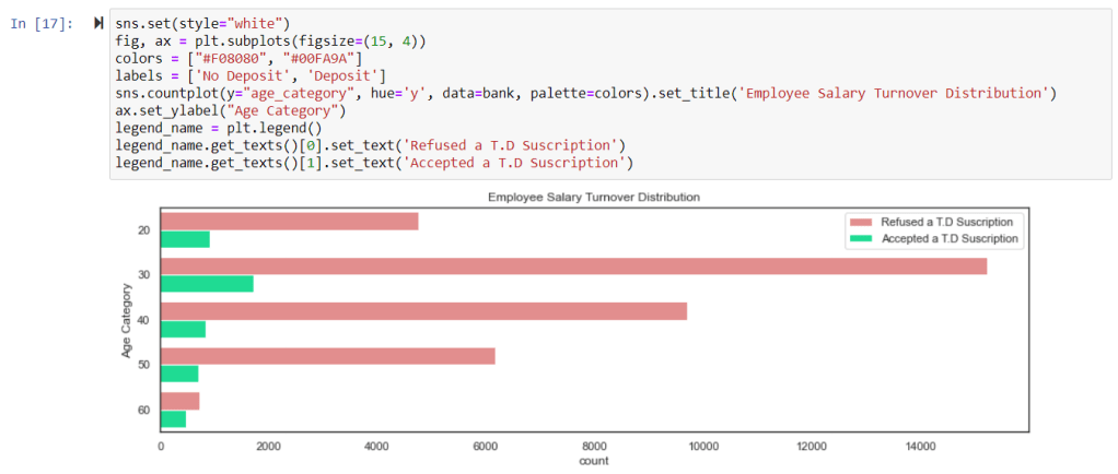
sns.set(style="white")
fig, ax = plt.subplots(figsize=(15, 4))
colors = ["#F08080", "#00FA9A"]
labels = ['No Deposit', 'Deposit']
sns.countplot(y="age_category", hue='y', data=bank, palette=colors).set_title('Employee Salary Turnover Distribution')
ax.set_ylabel("Age Category")
legend_name = plt.legend()
legend_name.get_texts()[0].set_text('Refused a T.D Suscription')
legend_name.get_texts()[1].set_text('Accepted a T.D Suscription')

Age Category vs Refused a term deposit | DSD — Age vs Subscription

sns.set(style="white")
fig, ax = plt.subplots(figsize=(14,8))
sns.countplot(x="job", data=bank, palette="Set1")
ax.set_title("Occupations of Potential Clients", fontsize=20)
ax.set_xlabel("Types of Jobs")
plt.show()

Occupations Distribution | DSD — Occupations Distribution

sns.set(style="white")
fig, ax = plt.subplots(figsize=(15, 8))
colors = ["#F08080", "#00FA9A"]
labels = ['No Deposit', 'Deposit']
sns.countplot(y="job", hue='y', data=bank, palette=colors).set_title('Employee Salary Turnover Distribution')
ax.set_ylabel("job")
legend_name = plt.legend()
legend_name.get_texts()[0].set_text('Refused a T.D Suscription')
legend_name.get_texts()[1].set_text('Accepted a T.D Suscription')

Job Type vs Subscription of Term Deposit | DSD — Job Type vs Subscription

Correlation Plot

corr = bank.corr()
sns.heatmap(corr,annot=True,cmap='RdYlGn',linewidths=0.2,annot_kws={'size':20})
fig=plt.gcf()
fig.set_size_inches(18,15)
plt.xticks(fontsize=14)
plt.yticks(fontsize=14)
plt.show()

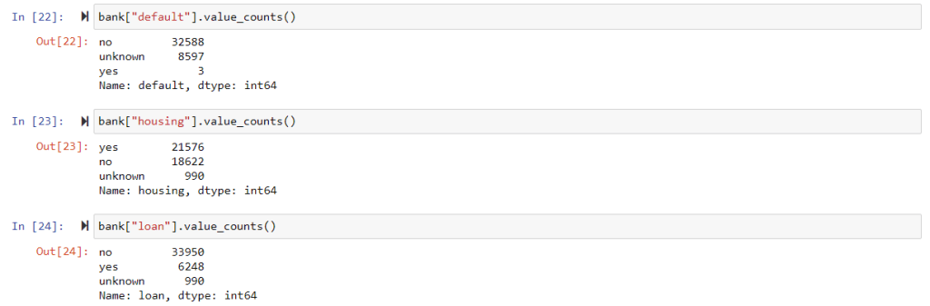
convert above columns to have numeric labels as 0 or 1.

bank["default"] = bank["default"].apply(lambda x: 0 if x == 'no' else 1)
bank["housing"] = bank["housing"].apply(lambda x: 0 if x == 'no' else 1)
bank["loan"] = bank["loan"].apply(lambda x: 0 if x == 'no' else 1)

convert duration in seconds to duration in minutes up to two decimal points.

 decimal_points = 2
 bank['duration'] = bank['duration'] / 60 #convert seconds to minute
 bank['duration'] = bank['duration'].apply(lambda x: round(x, decimal_points))

f,ax=plt.subplots(1,2,figsize=(18,8))
colors=["#F08080", "#00FA9A"]
labels = 'Refused a T.D. Suscription', 'Accepted a T.D. Suscription'
bank['y'].value_counts().plot.pie(explode=[0,0.1],autopct='%1.1f%%',ax=ax[0],
shadow=True, colors=colors, labels=labels,fontsize=14)
ax[0].set_title('Term Deposits', fontsize=20)
ax[0].set_ylabel('% of Total Potential Clients', fontsize=14)
sns.countplot('y',data=bank,ax=ax[1], palette=colors)
ax[1].set_title('Term Deposits', fontsize=20)
ax[1].set_xticklabels(['Refused', 'Accepted'], fontsize=14)
plt.show()

 
bank['year'] = 2017
 lst = [bank]
 Create a column with the numeric values of the months.
 for column in lst:
     column.loc[column["month"] == "jan", "month_int"] = 1
     column.loc[column["month"] == "feb", "month_int"] = 2
     column.loc[column["month"] == "mar", "month_int"] = 3
     column.loc[column["month"] == "apr", "month_int"] = 4
     column.loc[column["month"] == "may", "month_int"] = 5
     column.loc[column["month"] == "jun", "month_int"] = 6
     column.loc[column["month"] == "jul", "month_int"] = 7
     column.loc[column["month"] == "aug", "month_int"] = 8
     column.loc[column["month"] == "sep", "month_int"] = 9
     column.loc[column["month"] == "oct", "month_int"] = 10
     column.loc[column["month"] == "nov", "month_int"] = 11
     column.loc[column["month"] == "dec", "month_int"] = 12
 Change datatype from int32 to int64
 bank["month_int"] = bank["month_int"].astype(np.int64)
bank.drop(['day_of_week','year'], axis=1, inplace=True)

 
f, axes = plt.subplots(ncols=3, figsize=(15, 8))
 Graph Employee Satisfaction
 sns.distplot(bank['month_int'], kde=False, color="#ff3300", ax=axes[0]).set_title(
'Months of Marketing Activity Distribution')
 axes[0].set_ylabel('Potential Clients Count')
 axes[0].set_xlabel('Months')
 Graph Employee Evaluation
 sns.distplot(bank['age'], kde=False, color="#3366ff", ax=axes[1]).set_title(
'Age of Potentical Clients Distribution')
 axes[1].set_ylabel('Potential Clients Count')
 Campaigns
 sns.distplot(bank['campaign'], kde=False, color="#546E7A", ax=axes[2]).set_title(
'Calls Received in the Marketing Campaign')
 axes[2].set_ylabel('Potential Clients Count')
 plt.show()

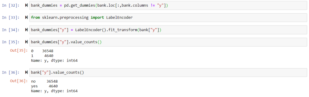
Convert Categorical Variables to Dummy Variables

 
# Dummy all categorical variables except the target one.
bank_dummies = pd.get_dummies(bank.loc[:,bank.columns != "y"])
#use label encoder for target variable
from sklearn.preprocessing import LabelEncoder
bank_dummies["y"] = LabelEncoder().fit_transform(bank["y"])

Train Test Split

Why stratified sampling?

It is used to eliminate sampling bias in a test set.
It allows to create a test set with a population that best represents the entire population being studied.
Stratified random sampling is different from simple random sampling, which involves the random selection of data from the entire population so that each possible sample is equally likely to occur.
If sampling bias occurs when building a test set then when testing a machine learning model it show that the model is performing poorly as the test set does not represent the whole population.

Advantages of Stratified Sampling

Stratified random sampling accurately reflects the population being studied.
It ensures each subgroup within the population receives proper representation within the sample.
As a result, stratified random sampling provides better coverage of the population.

 
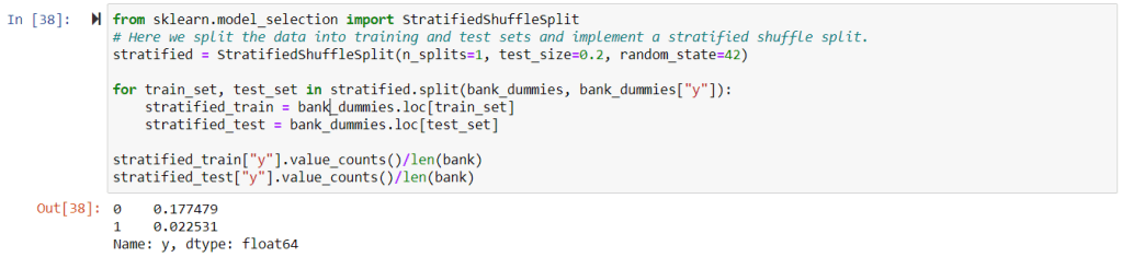
from sklearn.model_selection import StratifiedShuffleSplit
 # Here we split the data into training and test sets and 
# implement a stratified shuffle split.
 stratified = StratifiedShuffleSplit(n_splits=1, test_size=0.2, random_state=42)
 for train_set, test_set in stratified.split(bank_dummies, bank_dummies["y"]):
     stratified_train = bank_dummies.loc[train_set]
     stratified_test = bank_dummies.loc[test_set]
 stratified_train["y"].value_counts()/len(bank)
 stratified_test["y"].value_counts()/len(bank)

 
#Normal splitting with sklearn train test
#from sklearn.model_selection import train_test_split
 #X = train_data.drop('y',axis=1)
 #y = train_data['y']
 #X_train, X_test, y_train, y_test = train_test_split(X, y, test_size=0.30, #random_state=101)

X_train = train_data.drop('y',axis=1)
y_train = train_data['y']
X_test = test_data.drop('y',axis=1)
y_test = test_data['y']

There is un-even distribution of classes in target variable so will go for over sampling – SMOTE

print("Before OverSampling, counts of label '1': {}".format(
sum(y_train == 1))) 
print("Before OverSampling, counts of label '0': {} \n".format(
sum(y_train == 0)))

from imblearn.over_sampling import SMOTE 
sm = SMOTE(random_state = 2) 
X_train_res, y_train_res = sm.fit_resample(X_train, y_train.ravel())

print("After OverSampling, counts of label '1': {}".format(
sum(y_train_res == 1))) 
print("After OverSampling, counts of label '0': {} \n".format(
sum(y_train_res == 0)))

Training a Decision Tree Model

from sklearn.tree import DecisionTreeClassifier
DTClassifier = DecisionTreeClassifier()
DTClassifier.fit(X_train_res,y_train_res)
print("Train Accuracy:",DTClassifier.score(X_train_res, y_train_res))

predictions = DTClassifier.predict(X_test)
from sklearn.metrics import classification_report,confusion_matrix,accuracy_score
# Confusion matrix
print(confusion_matrix(y_test,predictions))
print("Test Accuracy:",DTClassifier.score(X_test, y_test))

Observation from the training and test accuracy scores

you can clearly see that the training accuracy is 1 that is 100% and testing accuracy is .88 that is 88%. this is the clear cut case of over fitting. Normally decision tree suffers with the problem of over fitting. As decision tree is nothing but the if else representation in tree form for each feature variables with respect to the target one. hence in general if we build base model of decision tree then it simply outperform on training data and will not be able to generalize the same behavior on test data.

To overcome the over fitting problem there are certain methods like pruning. Pruning happens in two ways one Pre-pruning that is decide the no of features before the tree is build and in second post pruning we build the whole tree first and then start cutting the nodes (features) from bottom up manner and in each cut check the accuracy. There are other methods like cross validation grid search and random search which I have explained in theory part of decision tree.

In this post I am focusing more on implementing those concepts as following.

from sklearn.model_selection import RandomizedSearchCV
from scipy.stats import randint
param_dist = {"max_depth": [3, None],
              "max_features": randint(1,50),
              "min_samples_leaf": randint(50,1000),
              "criterion": ["gini", "entropy"]}
#Instantiate a Decision Tree classifier: tree
tree = DecisionTreeClassifier()
#Instantiate the RandomizedSearchCV object: tree_cv
tree_cv = RandomizedSearchCV(tree, param_dist, cv=5)
#Fit it to the data
tree_cv.fit(X_train_res, y_train_res)
#Print the tuned parameters and score
print("Tuned Decision Tree Parameters: {}".format(tree_cv.best_params_))
print("Best score is {}".format(tree_cv.best_score_))

Decision Tree RandomizedSearchCV | DSD — Decision Tree RandomizedSearchCV

Here if you see then find that training accuracy is 88% and test accuracy is also near to 87%. And you see over fitting is clearly removed as both training and testing performance are in same level.

Note:

There are many other things to do as part of feature engineering and in data pre-processing. It all depends on domain understanding, problem understanding etc. So spend some time on understanding the problem and think what could be done with features and come up with the best possible model.
As you see Decision Tree is very prone to over fitting problem hence instead of using decision for any of the production code, it is advisable to explore Random Forest and other boosting methods like xgboost, adaboost etc.

So this is all in decision tree implementation using python. If you face any difficulty in any of the steps then please feel free to ask using the comment.