A Complete Guide to K-Nearest Neighbors Algorithm – KNN using Python

k-Nearest Neighbors or kNN algorithm is very easy and powerful Machine Learning algorithm. It can be used for both classification as well as regression that is predicting a continuous value. The very basic idea behind kNN is that it starts with finding out the k-nearest data points known as neighbors of the new data point for which we need to make the prediction. And then if it is regression then take the conditional mean of the neighbors y-value and that is the predicted value for new data point. If it is classification then it takes the mode (majority value) of the neighbors y value and that becomes the predicted class of the new data point.

In this article you will learn how to implement k-Nearest Neighbors or kNN algorithm from scratch using python. Problem described is to predict whether a person will take the personal loan or not. Data set used is from universal bank data set.

Table of Contents

1. The intuition behind KNN – understand with the help of a graph.
2. How KNN as an algorithm works?
3. How to find the k-Nearest Neighbors?
4. Deciding k – The hyper parameter in KNN.
5. Complete end to end example using python which includes
   • Exploratory data analysis
   • Imputing missing values
   • Data Pre-processing
   • Train Test split of data
   • Training the model using KNN
   • Predicting on test data
6. Additional Reading

The intuition behind KNN – understand with the help of a graph

Let’s start with one basic example and try to understand what is the intuition behind the KNN algorithm. Consider the following example containing a data frame with three columns Height, Age and weight. The values are randomly chosen.

import pandas as pd
import matplotlib.pyplot as plt
Age = [45,26,30,34,40,36,19,28,23,32,38]
Height = [5,5.11,5.6,5.9,4.8,5.8,5.3,5.8,5.5,5.6,5.5]
Weight = [77,47,55,59,72,60,40,60,45,58,"?"]
Height_Age_Weight_df = pd.DataFrame({"Height":Height,"Age":Age,"Weight":Weight})
Height_Age_Weight_df

So now the problem is to predict the weight of a person whose height is 5.50 feet and his age is 38 years (see the 10th row in data set). In the below scatter plot between Height and Age this test point is marked as “x” in blue color.

 
plt.scatter(Age, Height,color = 'r')
plt.xlabel('Age')
plt.ylabel('Height')
plt.show()
 

So if you look carefully the above scatter plot and observe that this test point is closer to the circled point. And hence it’s weight will be closer to the weight of these two persons. This is fair enough answer. So these circled points become the neighbors of the test data point. This is the exact idea behind the KNN algorithm.How KNN as an algorithm works?How KNN as an algorithm works?

How KNN as an algorithm works?

Let’s take one more example: Consider one Predictor variable x and Target variable y. And we want to predict value of y for x = 13. (See the data below)

 
x = [10,13.8,12.5,16,34,23,27,18,30,13]
y = [11,14.8,13.5,17,35,24,28,19,31,"?"]
random_df = pd.DataFrame({"X":x,"Y":y})
random_df

So we will look data points in x which are equal or closer to x= 13. Those are known as neighbors to the new data point. So these points are 12.5, 13.8 and 10 if we take k = 3 nearest neighbors. Now find selected neighbors corresponding y value those are 13.5, 14.8 and 11. Note k is hyper parameter and decision to take how many k’s will discuss in next heading.

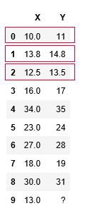
And take mean of those y values as (11+14.8+13.5)/3 = 13.1. So this will be the predicted value for new data point x = 13. Whether we will take mean or median or some other measures it depends on the Loss function. In case of L2 loss that is minimizing the squared error values, we take mean of y values and it is known as conditional mean. If our loss function is of L1 loss then we go with finding median of neighbors y values.

According to statistics “The best prediction of y at an point X = x is the conditional mean in case of L1 Loss and is conditional median in case of L1 Loss”.

This was the example of predicting a continuous value that is regression problem. KNN can also be used for classification problem. only the difference will be in this case, we will take the mode of neighbors y values that is taking the majority of y. For example in above case if we have neighbors y values as 1, 0, 1 then majority is 1 and hence we will predict our data point x = 13 will belong to class 1. This is how KNN can also be used for classification problems.

How to find the k-Nearest Neighbors?

To find the nearest neighbors, Algorithm calculates the distance between the new data point and training data points. And then shortlist the points which are closer to the new data point. These shortlisted points are known as the nearest neighbors to the new data point. Now two question arises how to calculate the distance between points and how many (k) closer points to be shortlisted. Decision of k will discuss in next heading, now let’s understand how to calculate the distance.

The most commonly used distance measures are Euclidean and Manhattan for continuous value prediction that is regression and Hamming Distance for categorical or classification problems.

1. Euclidean Distance

Euclidean distance is calculated as the square root of the sum of the squared differences between a new point (X2) and an existing point (X1).

2. Manhattan Distance

This is the distance between real vectors using the sum of their absolute difference.

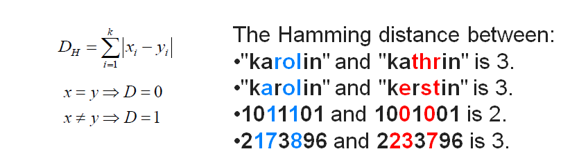
3. Hamming Distance

It is used for categorical variables. If the value (x) and the value (y) are same, the distance D will be equal to 0 . Otherwise D=1.

4. Deciding k – The hyper parameter in KNN

k is nothing but the number of nearest neighbors to be selected to finally predict the outcome of new data point. Decision of choosing the k is very important, although there is no mathematical formula to decide the k.

We start with some random value of k and then start increasing until it is reducing the error in predicted value. once it start increasing the error we stop there. Also overfitting case need to be taken care here. Sometime we end up choosing large value of k which best suited in training data but drastically increases the error in test or live data. Hence we divide the data in three parts train, validation and test. we select k based on train data and check if it is not overfitting by validating it against validation data.

This procedure required multiple iteration and then finally we get the best suited value of k. However this all we no need to do manually, we can write a function or utilize the inbuilt libraries in python which produces the final k value.

5. Complete end to end example using python

Problem Description

• In the following Supervised Learning activity, we try to predict those who will likely accept the offer of a new personal loan.
• ID: Customer ID
• Age: Customer’s age in completed years
• Experience: #years of professional experience
• Income: Annual income of the customer ($000)
• ZIPCode: Home Address ZIP code. Do not use ZIP code Family: Family size of the customer
• CCAvg: Avg. spending on credit cards per month ($000)
• Education: Education Level. 1: Undergrad; 2: Graduate; 3: Advanced/Professional
• Mortgage: Value of house mortgage if any. ($000)
• Personal Loan: Did this customer accept the personal loan offered in the last campaign?
• Securities Account: Does the customer have a securities account with the bank?
• CD Account: Does the customer have a certificate of deposit (CD) account with the bank?
• Online: Does the customer use internet banking facilities?
• CreditCard: Does the customer use a credit card issued by UniversalBank?

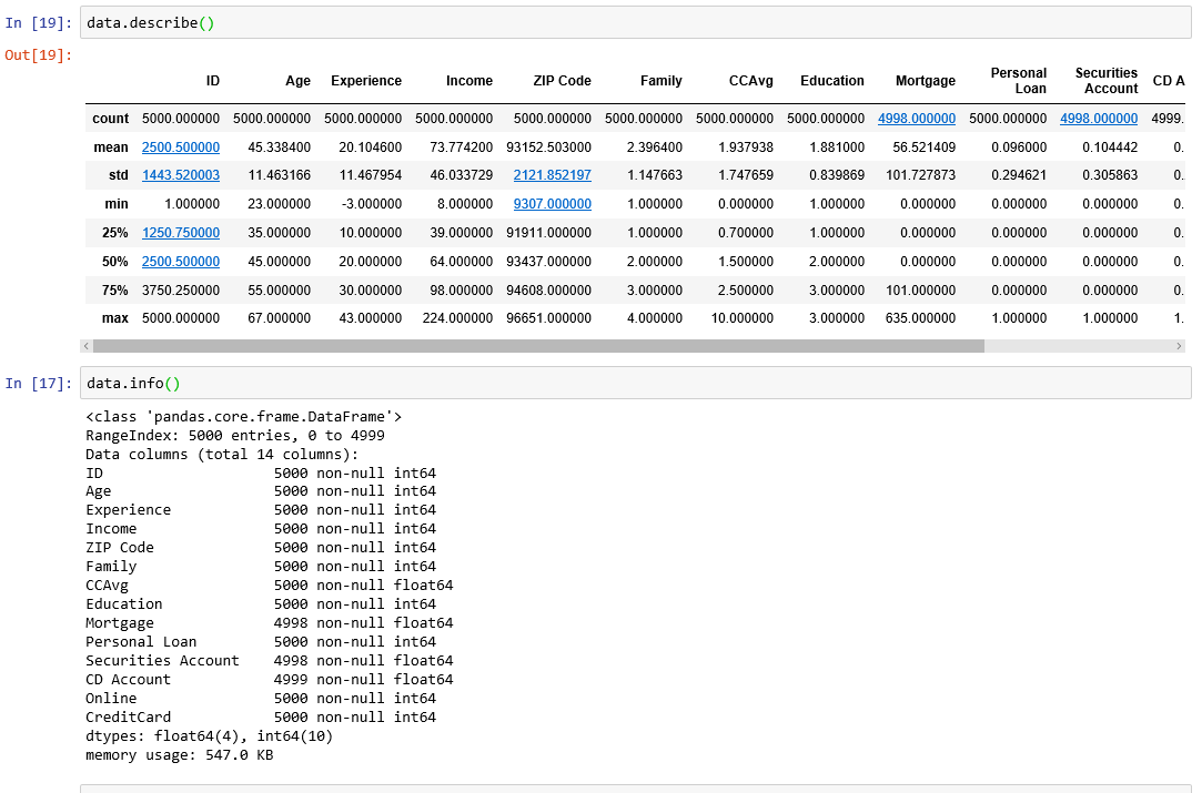
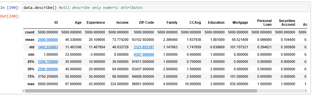
5.2 Exploratory data analysis

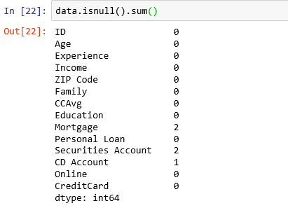
5.3 Imputing missing values

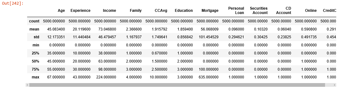
5.4 Data Pre-processing

5.5 Train Test split of data

from sklearn.model_selection import train_test_split
 X = data.drop('Personal Loan',axis=1).values
 y = data['Personal Loan'].values
 X_train,X_test,y_train,y_test = train_test_split(X,y,test_size=0.4,random_state=42, stratify=y) 

5.6 Decide K the number of nearest neighbors

 
 
 import KNeighborsClassifier
 from sklearn.neighbors import KNeighborsClassifier
 Setup arrays to store training and test accuracies
 neighbors = np.arange(1,15)
 train_accuracy =np.empty(len(neighbors))
 test_accuracy = np.empty(len(neighbors))
 for i,k in enumerate(neighbors):
     #Setup a knn classifier with k neighbors
     knn = KNeighborsClassifier(n_neighbors=k)
     #Fit the model 
     knn.fit(X_train, y_train) 
     #Compute accuracy on the training set 
     train_accuracy[i] = knn.score(X_train, y_train) 
     #Compute accuracy on the test set 
     test_accuracy[i] = knn.score(X_test, y_test) 
 

 
#Generate plot
 plt.title('k-NN Varying number of neighbors')
 plt.plot(neighbors, test_accuracy, label='Testing Accuracy')
 plt.plot(neighbors, train_accuracy, label='Training accuracy')
 plt.legend()
 plt.xlabel('Number of neighbors')
 plt.ylabel('Accuracy')
 plt.show()
 

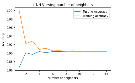
From the above plot we can say that we get maximum test accuracy for k = 8 and after that it is constant. Hence we will finalize k as 8 and train the model for 8 nearest neighbors.

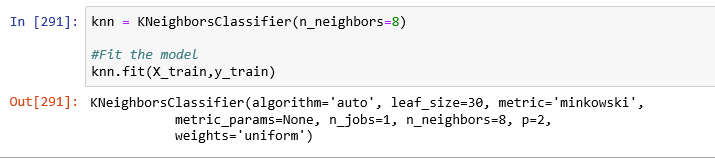
5.7 Training the model using KNN

#Setup a knn classifier with k neighbors
knn = KNeighborsClassifier(n_neighbors=8)

#Fit the model
knn.fit(X_train,y_train) 

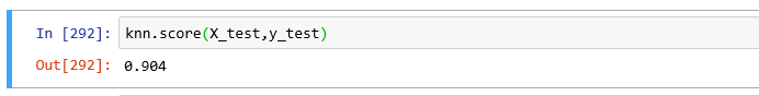
5.8 Predicting on test data

 
#Get accuracy. 
#Note: In case of classification algorithms score method 
#represents accuracy. 
knn.score(X_test,y_test) 

5.9 Confusion Matrix

A confusion matrix is a table that is often used to describe the performance of a classification model (or “classifier”) on a set of test data for which the true values are known. Scikit-learn provides facility to calculate confusion matrix using the confusion_matrix method.

#import confusion_matrix
from sklearn.metrics import confusion_matrix

<em>#let us get the predictions using the classifier we had fit above</em> 
y_pred = knn.predict(X_test) 

confusion_matrix(y_test,y_pred)

5.10 Classification Report

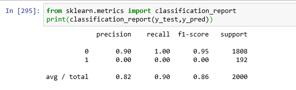
Another important report is the Classification report. It is a text summary of the precision, recall, F1 score for each class. Scikit-learn provides facility to calculate Classification report using the classification_report method.

 
<em>#import classification_report</em> 
from sklearn.metrics import classification_report
print(classification_report(y_test,y_pred))
 

Some Important Points

• KNN is Model free algorithm. As there is no assumption on form of function f. You see in regression at last we get a function in terms of x and y including coefficients and constant values.
• Computational complexity increases with increase in data set size
• It suffers with “Curse of Dimensionality” problem. Because when dimensions increases it produces less accuracy.
• Increase the neighbors, it creates smoother boundaries to classify correctly.

Improving (Speeding up) KNN

Clustering as a Pre processing Step

• Eliminate most points (keep only cluster centroids)
• Apply knn

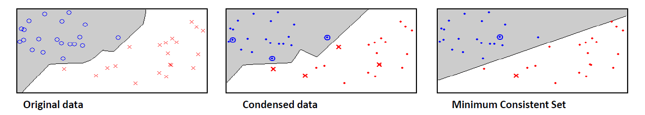
Condensed NN

• Retain samples closest to “decision boundaries”
• Decision Boundary Consistent – a subset whose nearest neighbor decision boundary is identical to the boundary of the entire training set
• Minimum Consistent Set – the smallest subset of the training data that correctly classifies all of the original training data

Reduced NN

• Remove a sample if doing so does not cause any incorrect classifications
• Initialize subset with a single training example
• Classify all remaining samples using the subset, and transfer any incorrectly classified samples to the subset
• Return to 2 until no transfers occurred or the subset is full

Recommended Articles:

• A Step by Step Guide to Logistic Regression Model Building using Python | Machine learning
• Reference Python Notebooks for Important ML Algorithms for the Beginners
• How to deploy machine learning models as a microservice using fastapi
• Machine Learning Interview questions and answers part 2 | ML Faq

Feel free to contact us for more details and discussions.