What is Linear Regression? Part:2

In any business there are some easy to measure variables like : Age, Gender, Income, Education Level etc. and there are some difficult to measure variables like amount of loan to give, no of days a patient will stay in the hospital, price of the house after 10 years etc. So Regression is the technique which enables you to determine difficult to measure variables with the help of easy to measure variables.

Linear Regression is one of the regression technique and can be defined as following:

“Linear Regression is a field of study which emphasizes on the statistical relationship between two continuous variables known as Predictor and Response variables”.
(Note: when there are more than one predictor variables then it becomes multiple linear regression.)

Predictor variable is most often denoted as x and also known as Independent variable.
Response variable is most often denoted as y and also known as Dependent variable.

Let’s understand it with the help of an example in R. There is a built-in data set “cars” available in R which contains 50 pairs of data points for speed(miles per hour mph) vs stopping distance (ft), that was collected in 1920. I took screenshot of first 25 data points for giving you a feel of data set.

In the above data set, if we see carefully we will find that for different cars for same speed there are different stopping distances. There could be multiple factors for this. Some factors could be different weather conditions, Tyre quality, car modal, road quality, traffic etc.

To understand Linear Regression, we are going to avoid all other factors and concentrate only on the speed of the car. So our objective is to find whether there exist any linear relationship between speed and stopping distance and will plot that relationship and then predict average stopping distance for all data points.

We can get some intuition about the relationship by observing Co-variance and Correlation coefficients as following:

Co-variance:

cov(cars_data$dist, cars_data$speed) #covariance
## [1] 109.9469

Co-variance between distance and speed is 109.9469 . It’s value is positive which tells us that variables are moving together in same direction. (Opposite to each other in case of negative value).

Correlation:

To know the strength of how the variables move together co-variance is standardized to the dimensionless quantity, correlation. Correlation coefficient r is a number between -1 to +1 which tells us how well a (regression) line fits the data.

cor(cars_data$speed, cars_data$dist)      # Correlation
## [1] 0.8068949

The correlation coefficient of the Speed of car and Distance is 0.8068949.
Since the value is close to 1 and has a +ve sign, we can conclude that the variables are positively correlated.

Recommended Article: Covariance and Correlation in detail

Let’s visualize the data set by drawing scatter plot.

Independent variable (Predictor variable) – Speed (mph) – plotted on X-axis.
Dependent variable (Response variable) – Stopping distance (ft) – plotted on Y-axis.

plot(cars_data$speed,cars_data$dist,xlab="Speed in miles per hour",ylab="Distance in feet",main="Stopping Distance Vs. Speed", col= "blue")

Scatter Plot to understand Linear Regression

Observations from the Scatter Plot:

At red mark point, there are multiple stopping distances for same speed. This could be possibly because of different cars, different roads, different weather condition etc.
So if we take the average of all those points at red mark then it will give the average stopping distance at that point but what if we want to know the stopping distance at yellow mark. We do not have any data given at this yellow point.
So instead of focusing on any local points if we take all the point and somehow impute the mean value at yellow marked point that would be stopping distance at that point.

How to do this, if we draw a straight line through all the data points which will give the sample mean of stopping distance as a function of speed.

This line equation will look like y = m*x + c m: slope and c: intercept at y

So if we change m and c then it will give us all the possible lines that we can draw.

To come to the conclusion we need to find the optimal values of slope m and intercept c which will produce the best fit line. So let’s understand what is the best fit line.

Best Fit Line:

So one could say, the line which passes through most no of data points is the best fit line. But now if we see in fig-01, shall we still say that it is the best fit line? No. if we remember our mid school days and being asked to draw a best fit line then we will draw a line similar to the orange line in fig-02. How our brain recognizes it as a best fit line. And surprisingly it does not passes through any of the data points. So how it is drawn, perhaps by joining the points which minimizes the distance from all the data points.

let’s understand some math behind it.

y is the actual value of data point x.
ŷ = m*x + c (ŷ is read as y-hat which is the predicted value of data point x using some m and c which we are trying to find out)

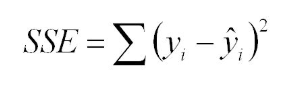
The difference y – ŷ is error term or also called as residual error. Considering all the data points this would be Σ (y(i) – ŷ(i)). This is known as average distance from all data points, which to be minimized, but by minimizing what do we mean. Do we consider the negative values of errors also, and if yes then if two data points have errors as +2 and -2 then they will be cancelled out while summing them up to calculate total error. So the best way to minimize the residuals error is to minimize the sum of squared error that is:

Now there are two unknowns m and c. so using calculus if we take the partial derivatives with respect to m and c and put them equal to 0 and solve the two equations we will get slope m as following:

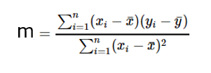
where xbar is the mean of x values and ybar is the mean of y values.

The intercept c can be computed by putting the (xbar, ybar) points to the equation y = m*x + c in place of x and y, as we know best fit line will pass through the mean points of x and y those are xbar and ybar. And the value of m is already computed.

This method of fitting the best line is called Least Square Regression

However in practical we do not need to compute all these manually, luckily we have R built-in functions to do it. let’s see those functions:

lm function is used to fit linear models

LinearReg = lm(dist ~ speed, data = cars_data)
coefficients(LinearReg)
##  (Intercept)      speed 
##  -17.579095    3.932409

## c = -17.579095
## m = 3.932409

## Summary of the linear model: 
summary(LinearReg)

## 
## Call:
## lm(formula = dist ~ speed, data = cars_data)
## 
## Residuals:
##     Min      1Q  Median      3Q     Max 
## -29.069  -9.525  -2.272   9.215  43.201 
## 
## Coefficients:
##             Estimate Std. Error t value Pr(>|t|)    
## (Intercept) -17.5791     6.7584  -2.601   0.0123 *  
## speed         3.9324     0.4155   9.464 1.49e-12 ***
## ---
## Signif. codes:  0 '***' 0.001 '**' 0.01 '*' 0.05 '.' 0.1 ' ' 1
## 
## Residual standard error: 15.38 on 48 degrees of freedom
## Multiple R-squared:  0.6511, Adjusted R-squared:  0.6438 
## F-statistic: 89.57 on 1 and 48 DF,  p-value: 1.49e-12

Let’s plot line of best fit using built-in function as following:

plot(cars_data$speed,cars_data$dist,xlab="Speed in miles per hour",ylab="Distance in feet",main="Stopping Distance Vs. Speed: Best fit line", col= "blue")
abline(LinearReg,col="steelblue",lty=1,lwd=4)       # The function adds straight line to a plot

So from above best fit line we can determine stopping distance for any data point from the population data. Linear Regression is very powerful technique to predict the value of a response variable when there is a Linear relationship between two continuous variable.

Please share your Ideas / thoughts in the comments section below.

Feel free to contact us for more details and discussions.