Frequently Asked Machine Learning Interview Questions from Linear Regression

1. What is Covariance coefficient?

Covariance tells you whether two random variables vary with respect to each other or not. And if they vary together then whether they vary in same direction or in opposite direction with respect to each other. So if both random variables vary in same direction then we say it is positive covariance, however if they vary in opposite direction then it is negative covariance.

Covariance Cov(X,Y) can be calculated as following:

Where:

x̄ is sample mean of x
ȳ is sample mean of y
x_i and y_i are the values of x and y for ith record in sample.
n is the no of records in sample

Significance of the formula:

Numerator: Quantity of variance in x multiplied by quantity of variance in y.
Unit of covariance: Unit of x multiplied by unit of y
Hence if we change the unit of variables, covariance will have new value however sign will remain same.
Therefore numerical value of covariance does not have any significance however if it is positive then both variables vary in same direction else if it is negative then they vary in opposite direction.

2. What is correlation coefficient?

As covariance only tells about the direction which is not enough to understand the relationship completely, we divide the covariance with standard deviation of x and y respectively and get correlation coefficient which varies between -1 to +1. It is denoted by ‘r’.

r = -1 and r= +1 tells that both variables have perfect linear relationship.
Negative means they are inversely proportional to each other with the factor of correlation coefficient value.
Positive means they are directly proportional to each other mean vary in same direction with the factor of correlation coefficient value.
if correlation coefficient is 0 then it means there is no linear relationship between variables however there could exist other functional relationship.
if there is no relationship at all between two variables then correlation coefficient will certainly be 0 however if it is 0 then we can only say that there is no linear relationship but there could exist other functional relationship.

Correlation between x and y can be calculated as following:

Where:

S_xy is the covariance between x and y.
S_x and S_y are the standard deviation of x and y respectively.
r_xy is correlation coefficient.
Correlation coefficient is dimensionless quantity. Hence if we change the unit of x and y then also coefficient value will remain same.

3. What is Multicollinearity? And how does it affect the linear regression?

Multicollinearity occurs in a multi linear model where we have more than one predictor variables. So Multicollinearity exist when we can linearly predict one predictor variable (note not the target variable) from other predictor variables with significant degree of accuracy. It means two or more predictor variables are highly correlated. But not the vice versa means if there is low correlation among predictors then also multicollinearity may exist.

Multicollinearity occurs when independent variables in a regression model are correlated. This is a problem because independent variables should be independent. If the degree of correlation between independent variables is high enough, it can cause problems when you fit the model.

A key goal of regression is to isolate the relationship between each independent variable and the dependent variable. The interpretation of a regression coefficient is that it represents the mean change in the dependent variable for each 1 unit change in an independent variable when you hold all of the other independent variables constant.

That last portion is crucial for our discussion about multicollinearity. The idea is that you can change the value of one independent variable and not the others. However, when independent variables are correlated, it indicates that changes in one variable are associated with shifts in another variable. The stronger the correlation, the more difficult it is to change one variable without changing another.

It becomes difficult for the model to estimate the relationship between each independent variable and the dependent variable independently because the independent variables tend to change in unison.

Hence Multicillinearity should be avoided in regression analysis. For more detailed explanation see: what-is-multicollinearity

4. What is Autocorrelation?

Autocorrelation refers to the degree of correlation between the values of the same variables across different observations in the data. The concept of autocorrelation is most often discussed in the context of time series data in which observations occur at different points in time (e.g., air temperature measured on different days of the month). For example, one might expect the air temperature on the 1st day of the month to be more similar to the temperature on the 2nd day compared to the 31st day.

If the temperature values that occurred closer together in time are, in fact, more similar than the temperature values that occurred farther apart in time, the data would be autocorrelated.

In a regression analysis, autocorrelation of the regression residuals can also occur if the model is incorrectly specified.

For example, if you are attempting to model a simple linear relationship but the observed relationship is non-linear (i.e., it follows a curved or U-shaped function), then the residuals will be autocorrelated.

5. What is Heteroscedasticity?

In regression analysis, we talk about heteroscedasticity in the context of the residuals or error term. If your error terms have varying variance rather than the constant variance, then we say its distribution is heteroscedastic.

Heteroscedasticity is a problem because ordinary least squares (OLS) regression assumes that all residuals are drawn from a population that has a constant variance (homoscedasticity).

6. How to check the strength of linearity between two continuous variables?

By simply plotting the scatter plot, you can visualize whether there is linear relationship between continuous variables or not. In case of linear relationship you will see there would be increasing or decreasing trend between those two variables as below:

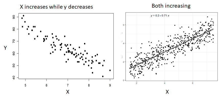
Linear Relationship check with scatter plot

You can also look for correlation value between these two variables. A high value of correlation coefficient (either in negative or positive) indicates the high linear relationship. Correlation coefficient value close to zero indicates weak linear relationship.

7. What is the significance of R-square or Coefficient of Determination value ?

Coefficient of determination is the measure of goodness of fit of the linear model. It can be defined as following:

R-square is the fraction (percentage) variation (change) in the response variable that is explainable by the predictor variables. In other words, how much variation in response variable is predicted by the predictor variables with the same level of accuracy. If R-square value is 84%, then we say that 84% variance in response variable is correctly predicted by the predictors with the help of the model. So your model is 84% accurate in predicting response variable.

R-square ranges between 0 (No Predictability) to 1 (100 % Predictability).

A high R-square indicates model is being able to predict response variable with less error.

Coefficient of determination is the most common way to measure the strength of the model mostly the linear model. More detail on how to calculate R-square value can be read here: what-is-the-coefficient-of-determination-r-square/

8. What is the difference between R-square and Adjusted R-Square values?

The adjusted R-squared is a modified version of R-squared that has been adjusted for the number of predictors in the model. The adjusted R-squared increases only if the new term improves the model more than would be expected by chance. It decreases when a predictor improves the model by less than expected by chance. The adjusted R-squared can be negative, but it’s usually not. It is always lower than the R-squared.

In the simplified Best Subsets Regression output below, you can see where the adjusted R-squared peaks, and then declines. Meanwhile, the R-squared continues to increase.

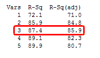
So if you see above screenshot carefully, then you will find that the value of r-square always increases with the increase in the number of predictors, however, adjusted r-square does not always increase. So in general adjusted r-square only increase if addition of new predictors bring more predictability to the model. Mean that new predictor has significant impact on target variable.

9. What are AIC and BIC values, seen at the output summary of Ordinary Least Square (OLs) in statsmodel?

The Akaike information criterion (AIC) is an estimator of prediction error and thereby relative quality of statistical models for a given set of data. Given a collection of models for the data, AIC estimates the quality of each model, relative to each of the other models. Thus, AIC provides a means for model selection.

When a statistical model is used to represent the process that generated the data, the representation will almost never be exact; so some information will be lost by using the model to represent the process. AIC estimates the relative amount of information lost by a given model: the less information a model loses, the higher the quality of that model.

In estimating the amount of information lost by a model, AIC deals with the trade-off between the goodness of fit of the model and the simplicity of the model. In other words, AIC deals with both the risk of overfitting and the risk of underfitting. we simply choose the model giving smallest AIC over the set of models considered.

In statistics, the Bayesian information criterion (BIC) or Schwarz information criterion (also SIC, SBC, SBIC) is a criterion for model selection among a finite set of models; the model with the lowest BIC is preferred. It is based, in part, on the likelihood function and it is closely related to the Akaike information criterion (AIC).

When fitting models, it is possible to increase the likelihood by adding parameters, but doing so may result in overfitting. Both BIC and AIC attempt to resolve this problem by introducing a penalty term for the number of parameters in the model; the penalty term is larger in BIC than in AIC.

10. What are the assumptions of Linear Regression?

There are four assumptions associated with a linear regression model:

Linearity: The relationship between X and the mean of Y is linear.
Homoscedasticity: The variance of residual is the same for any value of X. It mean no heteroscedasticity.
Independence: Observations (Predictors) are independent of each other. Also known as Multi collinearity. So there should be no or very less multi collinearity among the predictors.
Normality: For any fixed value of X, Y is normally distributed.
No auto-correlation: Target variable values should not be auto-correlated.

Refer for more detail: Linear Regression Assum ptions

11. How do you define the best fit line? How it is drawn?

In ordinary least squares (OLS) method, Line of best fit the one that minimizes the sum of squared differences between actual and predicted values. And it passes through the mean point of all the data points. Refer Linear Regression for more understanding on how to get coefficients and intercept to draw the best fit line: what-is-linear-regression-part

12. While calculating best fit line, why don’t we consider error as absolute difference of predicted vs actual values |Yactual – Ypredicted|? And why we consider Sum of Squared Error?

If we consider absolute error that mod of difference between actual and predicted values. it becomes mod function as |X| and it is not differentiable at x = 0. And hence we can not solve it to minimize the error and hence cant get the coefficient as well the intercept values. Hence we go for L2 norm that is squared differences between actual and predicted values. And then by taking partial derivatives with respect to betas we can easily get the coefficients values.

13. Is Linear Regression algorithm sensitive to outliers?

In the real world, data is often contaminated with outliers and poor quality data. If the number of outliers relative to non-outlier data points is more than a few, then the linear regression model will be skewed away from the true underlying relationship. And hence, we say that Linear Regression is sensitive to the outliers and before building the linear model, we should deal with outliers. One more reason is that outlier will deviate the line of best fit from the actual position where it should be and it would impact the predictive power.

14. What are techniques to identify outliers and how to handle them?

Most common causes of outliers on a data set:

Data entry errors (human errors)
Measurement errors (instrument errors)
Experimental errors (data extraction or experiment planning/executing errors)
Intentional (dummy outliers made to test detection methods)
Data processing errors (data manipulation or data set unintended mutations)
Sampling errors (extracting or mixing data from wrong or various sources)
Natural (not an error, novelties in data)

Identification of Outliers:

Box plot
Scatter plot
Z-score method
IQR score

Above methods are derived from the below techniques:

Extreme Value Analysis: Determine the statistical tails of the underlying distribution of the data. For example, statistical methods like the z-scores on univariate data.
Probabilistic and Statistical Models: Determine unlikely instances from a probabilistic model of the data. For example, gaussian mixture models optimized using expectation-maximization.
Linear Models: Projection methods that model the data into lower dimensions using linear correlations. For example, principle component analysis and data with large residual errors may be outliers.
Proximity-based Models: Data instances that are isolated from the mass of the data as determined by cluster, density or nearest neighbor analysis.
Information Theoretic Models: Outliers are detected as data instances that increase the complexity (minimum code length) of the dataset.
High-Dimensional Outlier Detection: Methods that search sub spaces for outliers give the breakdown of distance based measures in higher dimensions (curse of dimensionality).

Refer : how-to-identify-outliers-in-your-data

15. What do you understand by q-q plot in linear regression?

The q-q plot is used to answer the following questions:

Do two data sets come from populations with a common distribution?
Do two data sets have common location and scale?
Do two data sets have similar distributional shapes?
Do two data sets have similar tail behavior?

The quantile-quantile (q-q) plot is a graphical technique for determining if two data sets come from populations with a common distribution.

A q-q plot is a plot of the quantiles of the first data set against the quantiles of the second data set. By a quantile, we mean the fraction (or percent) of points below the given value. That is, the 0.3 (or 30%) quantile is the point at which 30% percent of the data fall below and 70% fall above that value.

A 45-degree reference line is also plotted. If the two sets come from a population with the same distribution, the points should fall approximately along this reference line. The greater the departure from this reference line, the greater the evidence for the conclusion that the two data sets have come from populations with different distributions.

The advantages of the q-q plot are:

The sample sizes do not need to be equal.
Many distributional aspects can be simultaneously tested. For example, shifts in location, shifts in scale, changes in symmetry, and the presence of outliers can all be detected from this plot. For example, if the two data sets come from populations whose distributions differ only by a shift in location, the points should lie along a straight line that is displaced either up or down from the 45-degree reference line.

The q-q plot is similar to a probability plot. For a probability plot, the quantiles for one of the data samples are replaced with the quantiles of a theoretical distribution.

This q-q plot of the JAHANMI2.DAT data set shows that

These 2 batches do not appear to have come from populations with a common distribution.
The batch 1 values are significantly higher than the corresponding batch 2 values.
The differences are increasing from values 525 to 625. Then the values for the 2 batches get closer again.

More reading on QQ Plot: linear-regression-plots-how-to-read-a-qq-plot

16. What is the significance of an F-test in a linear model?

In general, an F-test in regression compares the fits of different linear models. Unlike t-tests that can assess only one regression coefficient at a time, the F-test can assess multiple coefficients simultaneously.

The F-test of the overall significance is a specific form of the F-test. It compares a model with no predictors to the model that you specify. A regression model that contains no predictors is also known as an intercept-only model.

The hypotheses for the F-test of the overall significance are as follows:

Null hypothesis: The fit of the intercept-only model and your model are equal.
Alternative hypothesis: The fit of the intercept-only model is significantly reduced compared to your model.

In Minitab statistical software, you’ll find the F-test for overall significance in the Analysis of Variance table.

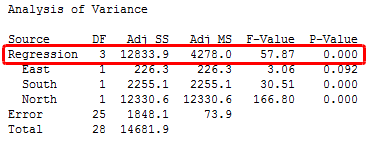
Analysis of variance table with the F-test of overall significance

If the P value for the F-test of overall significance test is less than your significance level, you can reject the null-hypothesis and conclude that your model provides a better fit than the intercept-only model.

If you don’t have any significant P values for the individual coefficients in your model, the overall F-test won’t be significant either. However, in a few cases, the tests could yield different results. For example, a significant overall F-test could determine that the coefficients are jointly not all equal to zero while the tests for individual coefficients could determine that all of them are individually equal to zero.

In the intercept-only model, all of the fitted values equal the mean of the response variable. Therefore, if the P value of the overall F-test is significant, your regression model predicts the response variable better than the mean of the response.

While R-squared provides an estimate of the strength of the relationship between your model and the response variable, it does not provide a formal hypothesis test for this relationship. The overall F-test determines whether this relationship is statistically significant. If the P value for the overall F-test is less than your significance level, you can conclude that the R-squared value is significantly different from zero.

17. What are the disadvantages of the linear model?

Linear Regression is limited to linear relationship
It is sensitive to outliers.
All predictors should be independent.

18. What is the use of Regularization? Explain L1 and L2 Regularization?

particularly in machine learning and inverse problems, regularization is the process of adding information in order to solve an ill-posed problem or to prevent overfitting.

Regularization are techniques used to reduce the error by fitting a function appropriately on the given training set and avoid overfitting.There are two important methods used in regularization are L1 (LASSO) Regularization and L2 (RIDGE) Regularization.

The main intuitive difference between the L1 and L2 regularization is that L1 regularization tries to estimate the median of the data while the L2 regularization tries to estimate the mean of the data to avoid overfitting.

L1 regularization adds the penalty term in cost function by adding the absolute value of weight(Wj) parameters, while L2 regularization adds the squared value of weights(Wj) in the cost function.

Ridge regression adds “squared magnitude” of coefficient as penalty term to the loss function. Here the highlighted part represents L2 regularization element.

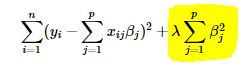
Here, if lambda is zero then you can imagine we get back OLS. However, if lambda is very large then it will add too much weight and it will lead to under-fitting. Having said that it’s important how lambda is chosen. This technique works very well to avoid over-fitting issue.

Lasso Regression (Least Absolute Shrinkage and Selection Operator) adds “absolute value of magnitude” of coefficient as penalty term to the loss function.

Again, if lambda is zero then we will get back OLS whereas very large value will make coefficients zero hence it will under-fit.

The key difference between these techniques is that Lasso shrinks the less important feature’s coefficient to zero thus, removing some feature altogether. So, this works well for feature selection in case we have a huge number of features.

19. How to choose the value of regularization parameter lambda in L1 and L2 regularization?

The regularization parameter (lambda) is an input to your model so what you probably want to know is how do you select the value of lambda. The regularization parameter reduces overfitting, which reduces the variance of your estimated regression parameters; however, it does this at the expense of adding bias to your estimate. Increasing lambda results in less overfitting but also greater bias. So the real question is “How much bias are you willing to tolerate in your estimate?”

One approach you can take is to randomly sub sample your data a number of times and look at the variation in your estimate. Then repeat the process for a slightly larger value of lambda to see how it affects the variability of your estimate. Keep in mind that whatever value of lambda you decide is appropriate for your sub sampled data, you can likely use a smaller value to achieve comparable regularization on the full data set.

Refer the link for more detailed understanding: how-to-calculate-the-regularization-parameter-in-linear-regression

20. What is robust regression?

A regression model should be robust in nature. This means that with changes in a few observations, the model should not change drastically. Also, it should not be much affected by the outliers.
A regression model with OLS (Ordinary Least Squares) is quite sensitive to the outliers. To overcome this problem, we can use the WLS (Weighted Least Squares) method to determine the estimators of the regression coefficients. Here, less weights are given to the outliers or high leverage points in the fitting, making these points less impactful.

21. When to do feature scaling after train test split or before the split?

In general, feature scaling should be done after split to avoid data leakage.

if we do scaling before the split, then training data will also have information about test data and hence model might not perform good when it comes to actual prediction on unseen data.
Data Leakage:
When information from outside the training data set is used to create the model. This can allow the model to learn or know something that it otherwise would not know and in turn invalidate the estimated performance of the model being constructed.

Preferred way:

Split data and Perform scaling separately in both training and testing set
Build model on training set.
Use the scaling parameters mean / variance from the training set to scale the testing data separately. Lets take example of standardization where we use standard deviation of training data to scale the features. So to scale test data use the same standard deviation and scale test data (than calculating standard deviation for testing data and use it.)
Then test on testing set.